Convolutional Neural Networks using Keras#
Machine Learning Methods#
Module 7: Neural Networks#
Part 3: Convolutional Neural Networks using Keras#
Instructor: Farhad Pourkamali#
Overview#
Convolutional Neural Networks (CNNs) capture spatial features from images, focusing on pixel arrangements and their relationships
Main Types of Layers:
Convolutional Layer: Extracts features using filters
Pooling Layer: Reduces the dimensionality and highlights dominant features
Fully-connected (FC) or Dense Layer: Combines features for final classification or regression
Advantages over Multilayer Perceptrons (MLPs):
Fewer parameters to learn due to shared weights in filters
Translation invariance: Treats all patches of the image uniformly, regardless of their position
Locality: Uses only small neighborhoods of pixels to compute hidden representations, making it computationally efficient
Example: The input is a two-dimensional tensor with a height of 3 and width of 3. The filter or kernel has a height of 2 and width of 2 (credit: Dive into Deep Learning, https://d2l.ai/)

A convolution layer is made up of a large number of convolution filters or kernels
A convolution filter relies on a simple operation, called a convolution
repeatedly multiplying matrix elements and then adding the results
consider a very simple example of a 4x3 image $\( \text{image}=\begin{bmatrix} a_{11} & a_{12} & a_{13} \\ a_{21} & a_{22} & a_{23} \\ a_{31} & a_{32} & a_{33} \\ a_{41} & a_{42} & a_{43} \\ \end{bmatrix} \)$
consider a 2x2 filter of the form $\( \text{filter}=\begin{bmatrix} f_{11} & f_{12} \\ f_{21} & f_{22} \\ \end{bmatrix} \)$
When we convolve the image with the filter, we get the result $\( \begin{bmatrix} a_{11}f_{11}+a_{12}f_{12}+a_{21}f_{21}+a_{22}f_{22} & a_{12}f_{11}+a_{13}f_{12}+a_{22}f_{21}+a_{23}f_{22}\\ a_{21}f_{11}+a_{22}f_{12}+a_{31}f_{21}+a_{32}f_{22} & a_{22}f_{11}+a_{23}f_{12}+a_{32}f_{21}+a_{33}f_{22}\\ a_{31}f_{11}+a_{32}f_{12}+a_{41}f_{21}+a_{42}f_{22} & a_{32}f_{11}+a_{33}f_{12}+a_{42}f_{21}+a_{43}f_{22}\\ \end{bmatrix} \)$
If the image size is \(n_h\times n_w\) and the size of the convolution filter is \(k_h\times k_w\), we get
Thus, the output size is slightly smaller than the input size
“Padding” refers to the technique of adding extra rows and columns of zeros around the input data before applying a convolution operation
control the spatial dimensions of the output feature maps
preserve information at the edges of the input
If we add a total of \(p_h\) rows of padding and \(p_w\) columns of padding, the output shape will be
Hence, we can give the input and output the same height and width by choosing
This is why CNNs commonly use convolution filters with odd height and width values
padding with the same number of rows on top and bottom, and the same number of columns on left and right
“Stride” controls how much the filter shifts (horizontally and vertically) between successive applications to generate the output feature map
That is, the number of rows and columns traversed per slide
A stride of 1 means that the filter moves one pixel at a time (no skipping)
A stride greater than 1 causes the filter to skip pixels
Example: strides of 3 and 2 for height and width (credit: Dive into Deep Learning, https://d2l.ai/)

Multiple input channels#
When the input data or image contains multiple channels, we need to construct a convolution filter with the same number of channels
For example, consider \(C\) channels for the previous case study, \(i=1,2,\ldots,C\)
\begin{equation}\text{channel \(i\) of image} =\begin{bmatrix} a_{11}^{(i)} & a_{12}^{(i)} & a_{13}^{(i)} \ a_{21}^{(i)} & a_{22}^{(i)} & a_{23}^{(i)} \ a_{31}^{(i)} & a_{32}^{(i)} & a_{33}^{(i)} \ a_{41}^{(i)} & a_{42}^{(i)} & a_{43}^{(i)} \ \end{bmatrix}\end{equation}
\begin{equation}\text{channel \(i\) of filter}=\begin{bmatrix} f_{11}^{(i)} & f_{12}^{(i)} \ f_{21}^{(i)} & f_{22}^{(i)} \ \end{bmatrix}\end{equation}
Final result: two-dimensional tensor
\begin{equation}\begin{bmatrix} \sum_{i=1}^C [a_{11}^{(i)}f_{11}^{(i)}+a_{12}^{(i)}f_{12}^{(i)}+a_{21}^{(i)}f_{21}^{(i)}+a_{22}^{(i)}f_{22}^{(i)}] & \sum_{i=1}^C [a_{12}^{(i)}f_{11}^{(i)}+a_{13}^{(i)}f_{12}^{(i)}+a_{22}^{(i)}f_{21}^{(i)}+a_{23}^{(i)}f_{22}^{(i)}]\ \sum_{i=1}^C [a_{21}^{(i)}f_{11}^{(i)}+a_{22}^{(i)}f_{12}^{(i)}+a_{31}^{(i)}f_{21}^{(i)}+a_{32}^{(i)}f_{22}^{(i)}] & \sum_{i=1}^C [a_{22}^{(i)}f_{11}^{(i)}+a_{23}^{(i)}f_{12}^{(i)}+a_{32}^{(i)}f_{21}^{(i)}+a_{33}^{(i)}f_{22}^{(i)}]\ \sum_{i=1}^C [a_{31}^{(i)}f_{11}^{(i)}+a_{32}^{(i)}f_{12}^{(i)}+a_{41}^{(i)}f_{21}^{(i)}+a_{42}^{(i)}f_{22}^{(i)}] & \sum_{i=1}^C [a_{32}^{(i)}f_{11}^{(i)}+a_{33}^{(i)}f_{12}^{(i)}+a_{42}^{(i)}f_{21}^{(i)}+a_{43}^{(i)}f_{22}^{(i)}]\ \end{bmatrix}\end{equation}
Example (credit: Dive into Deep Learning, https://d2l.ai/)

Multiple output channels#
In a convolution layer, you typically have multiple filters. Each filter is a small, learnable tensor that slides or convolves over the input data
The number of filters you specify in a layer determines the number of output channels
Denote by \(C_i\) and \(C_o\) the number of input and output channels
Let \(k_h\) and \(k_w\) be the height and width of the filter
To get an output with multiple channels, we can create a filter tensor of shape \(k_h\times k_w \times C_i\) for every output channel
Hence, we concatenate them on the output channel dimension, so that the shape of the convolution filter is \(k_h\times k_w \times C_i \times C_o\)
Example (credit: Dive into Deep Learning, https://d2l.ai/)
Maximum pooling#
The primary purpose of max pooling is to downsample the spatial dimensions of feature maps
This reduction in spatial resolution helps control the computational complexity of the network
Max pooling introduces a degree of position invariance, meaning that the model can recognize features regardless of their precise location in the input
In each pooling window (typically 2x2 or 3x3), max pooling selects the maximum value
It operates on each channel (feature map) of the input independently
Example (credit: Dive into Deep Learning, https://d2l.ai/)

import numpy as np
import keras
from keras import layers
# Model / data parameters
num_classes = 10
input_shape = (28, 28, 1)

# Load the data and split it between train and test sets
(x_train, y_train), (x_test, y_test) = keras.datasets.mnist.load_data()

# Scale images to the [0, 1] range
x_train = x_train.astype("float32") / 255
x_test = x_test.astype("float32") / 255

# Make sure images have shape (28, 28, 1)
x_train = np.expand_dims(x_train, -1)
x_test = np.expand_dims(x_test, -1)
print("x_train shape:", x_train.shape)
print(x_train.shape[0], "train samples")
print(x_test.shape[0], "test samples")


# convert class vectors to binary class matrices
y_train = keras.utils.to_categorical(y_train, num_classes)
y_test = keras.utils.to_categorical(y_test, num_classes)
x_train shape: (60000, 28, 28, 1)
60000 train samples
10000 test samples
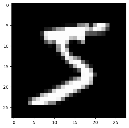
print(y_train[0])
[0. 0. 0. 0. 0. 1. 0. 0. 0. 0.]
import matplotlib.pyplot as plt

plt.imshow(x_train[0], cmap='gray')
<matplotlib.image.AxesImage at 0x333aeb110>
model = keras.Sequential(
    [
        keras.Input(shape=input_shape),
        layers.Conv2D(32, kernel_size=(3, 3), activation="relu"),
        layers.MaxPooling2D(pool_size=(2, 2)),
        layers.Conv2D(64, kernel_size=(3, 3), activation="relu"),
        layers.MaxPooling2D(pool_size=(2, 2)),
        layers.Flatten(),
        layers.Dropout(0.5),
        layers.Dense(num_classes, activation="softmax"),
    ]
)

model.summary()
2026-01-12 14:07:29.163925: I metal_plugin/src/device/metal_device.cc:1154] Metal device set to: Apple M2 Max
2026-01-12 14:07:29.164007: I metal_plugin/src/device/metal_device.cc:296] systemMemory: 64.00 GB
2026-01-12 14:07:29.164027: I metal_plugin/src/device/metal_device.cc:313] maxCacheSize: 24.00 GB
2026-01-12 14:07:29.164117: I tensorflow/core/common_runtime/pluggable_device/pluggable_device_factory.cc:305] Could not identify NUMA node of platform GPU ID 0, defaulting to 0. Your kernel may not have been built with NUMA support.
2026-01-12 14:07:29.164157: I tensorflow/core/common_runtime/pluggable_device/pluggable_device_factory.cc:271] Created TensorFlow device (/job:localhost/replica:0/task:0/device:GPU:0 with 0 MB memory) -> physical PluggableDevice (device: 0, name: METAL, pci bus id: <undefined>)
Model: "sequential"
┏━━━━━━━━━━━━━━━━━━━━━━━━━━━━━━━━━┳━━━━━━━━━━━━━━━━━━━━━━━━┳━━━━━━━━━━━━━━━┓
┃ Layer (type)                    ┃ Output Shape           ┃       Param # ┃
┡━━━━━━━━━━━━━━━━━━━━━━━━━━━━━━━━━╇━━━━━━━━━━━━━━━━━━━━━━━━╇━━━━━━━━━━━━━━━┩
│ conv2d (Conv2D)                 │ (None, 26, 26, 32)     │           320 │
├─────────────────────────────────┼────────────────────────┼───────────────┤
│ max_pooling2d (MaxPooling2D)    │ (None, 13, 13, 32)     │             0 │
├─────────────────────────────────┼────────────────────────┼───────────────┤
│ conv2d_1 (Conv2D)               │ (None, 11, 11, 64)     │        18,496 │
├─────────────────────────────────┼────────────────────────┼───────────────┤
│ max_pooling2d_1 (MaxPooling2D)  │ (None, 5, 5, 64)       │             0 │
├─────────────────────────────────┼────────────────────────┼───────────────┤
│ flatten (Flatten)               │ (None, 1600)           │             0 │
├─────────────────────────────────┼────────────────────────┼───────────────┤
│ dropout (Dropout)               │ (None, 1600)           │             0 │
├─────────────────────────────────┼────────────────────────┼───────────────┤
│ dense (Dense)                   │ (None, 10)             │        16,010 │
└─────────────────────────────────┴────────────────────────┴───────────────┘
Total params: 34,826 (136.04 KB)
Trainable params: 34,826 (136.04 KB)
Non-trainable params: 0 (0.00 B)
batch_size = 128
epochs = 15

model.compile(loss="categorical_crossentropy", optimizer="adam", metrics=["accuracy"])

model.fit(x_train, y_train, batch_size=batch_size, epochs=epochs, validation_split=0.1)
Epoch 1/15
2026-01-12 14:07:32.558642: I tensorflow/core/grappler/optimizers/custom_graph_optimizer_registry.cc:117] Plugin optimizer for device_type GPU is enabled.
422/422 ━━━━━━━━━━━━━━━━━━━━ 8s 11ms/step - accuracy: 0.7718 - loss: 0.7651 - val_accuracy: 0.9777 - val_loss: 0.0833
Epoch 2/15
422/422 ━━━━━━━━━━━━━━━━━━━━ 4s 10ms/step - accuracy: 0.9648 - loss: 0.1189 - val_accuracy: 0.9832 - val_loss: 0.0584
Epoch 3/15
422/422 ━━━━━━━━━━━━━━━━━━━━ 4s 10ms/step - accuracy: 0.9729 - loss: 0.0884 - val_accuracy: 0.9870 - val_loss: 0.0468
Epoch 4/15
422/422 ━━━━━━━━━━━━━━━━━━━━ 5s 11ms/step - accuracy: 0.9785 - loss: 0.0698 - val_accuracy: 0.9875 - val_loss: 0.0429
Epoch 5/15
422/422 ━━━━━━━━━━━━━━━━━━━━ 4s 10ms/step - accuracy: 0.9804 - loss: 0.0613 - val_accuracy: 0.9903 - val_loss: 0.0370
Epoch 6/15
422/422 ━━━━━━━━━━━━━━━━━━━━ 4s 10ms/step - accuracy: 0.9830 - loss: 0.0545 - val_accuracy: 0.9902 - val_loss: 0.0361
Epoch 7/15
422/422 ━━━━━━━━━━━━━━━━━━━━ 4s 10ms/step - accuracy: 0.9849 - loss: 0.0495 - val_accuracy: 0.9913 - val_loss: 0.0311
Epoch 8/15
422/422 ━━━━━━━━━━━━━━━━━━━━ 4s 10ms/step - accuracy: 0.9839 - loss: 0.0493 - val_accuracy: 0.9918 - val_loss: 0.0323
Epoch 9/15
422/422 ━━━━━━━━━━━━━━━━━━━━ 4s 10ms/step - accuracy: 0.9862 - loss: 0.0420 - val_accuracy: 0.9917 - val_loss: 0.0298
Epoch 10/15
422/422 ━━━━━━━━━━━━━━━━━━━━ 4s 10ms/step - accuracy: 0.9863 - loss: 0.0427 - val_accuracy: 0.9920 - val_loss: 0.0292
Epoch 11/15
422/422 ━━━━━━━━━━━━━━━━━━━━ 4s 10ms/step - accuracy: 0.9873 - loss: 0.0381 - val_accuracy: 0.9922 - val_loss: 0.0291
Epoch 12/15
422/422 ━━━━━━━━━━━━━━━━━━━━ 4s 10ms/step - accuracy: 0.9885 - loss: 0.0365 - val_accuracy: 0.9913 - val_loss: 0.0295
Epoch 13/15
422/422 ━━━━━━━━━━━━━━━━━━━━ 4s 10ms/step - accuracy: 0.9888 - loss: 0.0340 - val_accuracy: 0.9932 - val_loss: 0.0293
Epoch 14/15
422/422 ━━━━━━━━━━━━━━━━━━━━ 4s 10ms/step - accuracy: 0.9891 - loss: 0.0342 - val_accuracy: 0.9925 - val_loss: 0.0280
Epoch 15/15
422/422 ━━━━━━━━━━━━━━━━━━━━ 5s 11ms/step - accuracy: 0.9897 - loss: 0.0307 - val_accuracy: 0.9925 - val_loss: 0.0296
<keras.src.callbacks.history.History at 0x333ae8f10>
score = model.evaluate(x_test, y_test, verbose=0)
print("Test loss:", score[0])
print("Test accuracy:", score[1])
Test loss: 0.024686934426426888
Test accuracy: 0.991100013256073