Mathematical Building Blocks of Neural Networks#
Machine Learning Methods#
Module 7: Neural Networks#
Part 1: Mathematical Building Blocks of Neural Networks#
Instructor: Farhad Pourkamali#
Overview#
So far, we have seen two linear models for regression and classification problems
Linear regression: \(p(y|\mathbf{x},\mathbf{w})=\mathcal{N}(\mathbf{w}^T\mathbf{x}, \epsilon)\), where \(\epsilon\) is a fixed variance for all inputs
Logistic regression: \(p(y|\mathbf{x},\mathbf{w})=\text{Ber}(y|\sigma(\mathbf{w}^T\mathbf{x}))\), where \(\sigma\) is the sigmoid or logistic function
These models make the strong assumption that the input-output mapping is linear
A better idea: we can equip the feature extractor with its own “trainable” parameters
\[\mathbf{w}^T\phi(\mathbf{x};\boldsymbol{\theta})\]Illustrative example in the next slide!
Example, part 1: feature extractor#
Consider a classification problem with 3 input features \(x_1,x_2,x_3\)

Example, part 2: classifier#
This is the key idea behind multilayer perceptron (MLP) for “structured” or “tabular” data \(\mathbf{x}\in\mathbb{R}^D\)

1. Feedforward networks#
The information flows through the function being evaluated from \(\mathbf{x}\), through the intermediate computations, and finally to the output
For example, we might have \(f^{(1)}, f^{(2)}, f^{(3)}\) connected in a chain to form
\(f^{(1)}\): the first layer, \(f^{(2)}\): the second layer of the network
Because the training data does not show the desired output for these layers, they are called hidden layers
The overall length of the chain gives the depth, and the dimensionality of hidden layers determines the width of the model
Classical example: The XOR problem#
Learn a function that computes the exclusive OR of its two binary outputs (4 data points in \(\mathbb{R}^2\))
First activation function: \(g(z)=\text{ReLU}(z)=\max\{0,z\}\) and no activation function for the last layer

Classical example: The XOR problem#
This network correctly predicts all four class labels

Why nonlinear activation functions?#
If we just use a linear activation function, then the whole model reduces to a regular linear model
Therefore, it is important to use nonlinear activation functions
Sigmoid (logistic) function: \(\sigma(a)=\frac{1}{1+\exp(-a)}\)
rectified linear unit or ReLU: \(\text{ReLU}(a)=\max\{0, a\}\)
…
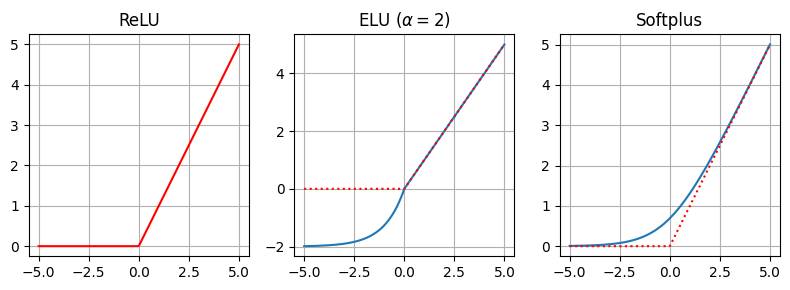
2. A tour of activation functions#
ReLU (Rectified Linear Unit)
ReLU is known for its simplicity and has been widely used in deep learning due to its ability to introduce non-linearity into the network
\[\text{ReLU}(x)=\max\{0, x\}\]ELU (Exponential Linear Unit)
ELU addresses the “dying ReLU” problem by allowing negative values, which helps to keep gradients flowing during training
\(\alpha\) is a hyperparameter that controls the output of the function for negative values of \(x\)
\[\begin{split}\text{ELU}(x)=\begin{cases}x & \text{if } x \geq 0 \\ \alpha \cdot \big(\exp(x) - 1\big) & \text{if } x < 0 \end{cases}\end{split}\]Softplus
Softplus is a smooth approximation of the ReLU function
It has the advantage of being differentiable everywhere, which makes it suitable for gradient-based optimization algorithms
\[\text{Softplus}(x)=\log\big(1+\exp(x)\big)\]
import numpy as np
import matplotlib.pyplot as plt

# Define a range of x values
x = np.linspace(-5, 5, 200)  # Adjust the range as needed

# Define the ReLU function
def relu(x):
    return np.maximum(0, x)

# Define the ELU function
def elu(x, alpha=2.0):
    return np.where(x >= 0, x, alpha * (np.exp(x) - 1))

# Define the Softplus function
def softplus(x):
    return np.log(1 + np.exp(x))


# Plot the activation functions
plt.figure(figsize=(8, 3))

plt.subplot(1, 3, 1)
plt.title("ReLU")
plt.plot(x, relu(x), 'r-')
plt.grid()

plt.subplot(1, 3, 2)
plt.title(r"ELU ($\alpha=2$)")
plt.plot(x, elu(x))
plt.plot(x, relu(x), 'r:')
plt.grid()

plt.subplot(1, 3, 3)
plt.title("Softplus")
plt.plot(x, softplus(x))
plt.plot(x, relu(x), 'r:')
plt.grid()

plt.tight_layout()
plt.show()