Building Neural Networks in Keras

Building Neural Networks in Keras#

Machine Learning Methods#

Module 7: Neural Networks#

Part 2: Building Neural Networks in Keras#

Instructor: Farhad Pourkamali#

Video: https://youtu.be/cXTHzXXuZlc

Gradient-based learning#

Neural networks are usually trained by using iterative, gradient-based optimizers such as (stochastic) gradient descent

\[\boldsymbol{\theta}_{t+1}=\boldsymbol{\theta}_{t} - \eta_t \nabla J(\boldsymbol{\theta}_{t})\]

\(\boldsymbol{\theta}_{t}\) is the parameter vector at iteration \(t\)
\(\eta_t\) is the learning rate, determining the step size
\(g_t=\nabla J(\boldsymbol{\theta}_{t})\) is the gradient of the loss function

1. Backprop#

Backpropagation is the core algorithm used for training neural networks through gradient-based optimization.
It enables the information from the loss function (or cost) to flow backward through the network—from the output layer to the input layer—in order to compute the gradients of the loss with respect to all trainable parameters (weights and biases).
This is achieved efficiently using the chain rule from calculus, which allows the computation of derivatives for functions composed of many layers or nested functions.
By recursively applying the chain rule from the output layer to the input layer, we obtain the gradients needed to update the model parameters via an optimization algorithm like gradient descent.

Backprop and chain rule#

Consider a 3-layer network with one unit in each layer and a scalar input

import tensorflow as tf

# Define the function f(u, v)
def f(u, v):
    return 3 * u + 5 * v

# Define values for x and y
x = tf.constant(2.0)
y = tf.constant(3.0)

# Use tf.GradientTape to compute gradients
with tf.GradientTape(persistent=True) as tape:
    # Watch the variables we want to compute gradients with respect to
    tape.watch(x)
    tape.watch(y)
    
    # Define u and v as functions of x and y
    u = 2 * x
    v = x + y

    # Define f as a function of u and v
    result = f(u, v)

# Compute the gradients
df_dx = tape.gradient(result, x)
df_dy = tape.gradient(result, y)


# Print the gradients
print("df/dx:", df_dx.numpy())
print("df/dy:", df_dy.numpy())

df/dx: 11.0
df/dy: 5.0

2. Implementing MLPs with Keras#

Keras is a high-level Deep Learning API to build, train, and evaluate all sorts of neural networks
- Keras runs on top of TensorFlow 2
- The best way to learn Keras: https://keras.io/
  - Layers
  - Models: groups layers into an object with training/inference features
  - Optimizers
  - Losses
  - Metrics

import numpy as np 
import pandas as pd
import matplotlib.pyplot as plt 
import tensorflow as tf
from tensorflow import keras

print(tf.__version__)

2.17.0

from sklearn.datasets import make_blobs

# Set random seed for reproducibility
np.random.seed(42)

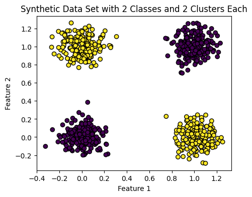
# Create synthetic data set
X, y = make_blobs(n_samples=800, centers=[[0, 0], [0, 1], [1, 0], [1, 1]], cluster_std=.1, random_state=42)

y[y == 0] = 0
y[y == 1] = 1
y[y == 2] = 1
y[y == 3] = 0


# Plot the synthetic data
plt.rcParams["figure.figsize"] = (5,4)
plt.scatter(X[:, 0], X[:, 1], c=y, cmap='viridis', edgecolors='k')
plt.title('Synthetic Data Set with 2 Classes and 2 Clusters Each')
plt.xlabel('Feature 1')
plt.ylabel('Feature 2')
plt.show()

../_images/5a7f3df0430463d6799df6e93d54fbdf3457532415d41accae74091253bd350f.png

from tensorflow.keras.models import Sequential
from tensorflow.keras.layers import Dense

# Define the model
model = Sequential()

# Add the input layer and the hidden layer
model.add(Dense(units=2, activation='relu', input_dim=2))  # Assuming 2 input features

# Add the output layer
model.add(Dense(units=1, activation='sigmoid'))  # Assuming binary classification

# Compile the model
model.compile(optimizer=tf.keras.optimizers.SGD(learning_rate=0.1), 
              loss='binary_crossentropy', metrics=['accuracy'])

# Display the model summary
model.summary()

/Users/farhad/anaconda3/lib/python3.10/site-packages/keras/src/layers/core/dense.py:87: UserWarning: Do not pass an `input_shape`/`input_dim` argument to a layer. When using Sequential models, prefer using an `Input(shape)` object as the first layer in the model instead.
  super().__init__(activity_regularizer=activity_regularizer, **kwargs)

Model: "sequential"

┏━━━━━━━━━━━━━━━━━━━━━━━━━━━━━━━━━┳━━━━━━━━━━━━━━━━━━━━━━━━┳━━━━━━━━━━━━━━━┓
┃ Layer (type)                    ┃ Output Shape           ┃       Param # ┃
┡━━━━━━━━━━━━━━━━━━━━━━━━━━━━━━━━━╇━━━━━━━━━━━━━━━━━━━━━━━━╇━━━━━━━━━━━━━━━┩
│ dense (Dense)                   │ (None, 2)              │             6 │
├─────────────────────────────────┼────────────────────────┼───────────────┤
│ dense_1 (Dense)                 │ (None, 1)              │             3 │
└─────────────────────────────────┴────────────────────────┴───────────────┘

 Total params: 9 (36.00 B)

 Trainable params: 9 (36.00 B)

 Non-trainable params: 0 (0.00 B)

model.layers[0].get_weights()

[array([[-0.01123536, -0.47319353],
        [ 1.1767792 ,  1.1020399 ]], dtype=float32),
 array([0., 0.], dtype=float32)]

model.layers[1].get_weights()

[array([[-0.05708301],
        [ 1.0786306 ]], dtype=float32),
 array([0.], dtype=float32)]

model.layers[2].get_weights()

---------------------------------------------------------------------------
IndexError                                Traceback (most recent call last)
Cell In[8], line 1
----> 1 model.layers[2].get_weights()

IndexError: list index out of range

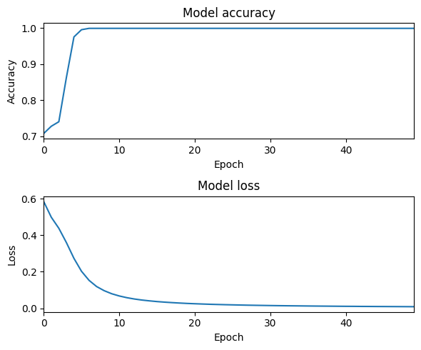
history = model.fit(X, y, epochs=50, batch_size=8)

Epoch 1/50
100/100 ━━━━━━━━━━━━━━━━━━━━ 0s 2ms/step - accuracy: 0.6552 - loss: 0.6233
Epoch 2/50
100/100 ━━━━━━━━━━━━━━━━━━━━ 0s 2ms/step - accuracy: 0.7253 - loss: 0.5177
Epoch 3/50
100/100 ━━━━━━━━━━━━━━━━━━━━ 0s 2ms/step - accuracy: 0.7158 - loss: 0.4608
Epoch 4/50
100/100 ━━━━━━━━━━━━━━━━━━━━ 0s 2ms/step - accuracy: 0.8179 - loss: 0.3631
Epoch 5/50
100/100 ━━━━━━━━━━━━━━━━━━━━ 0s 2ms/step - accuracy: 0.9678 - loss: 0.2753
Epoch 6/50
100/100 ━━━━━━━━━━━━━━━━━━━━ 0s 2ms/step - accuracy: 0.9955 - loss: 0.2081
Epoch 7/50
100/100 ━━━━━━━━━━━━━━━━━━━━ 0s 2ms/step - accuracy: 0.9977 - loss: 0.1683
Epoch 8/50
100/100 ━━━━━━━━━━━━━━━━━━━━ 0s 2ms/step - accuracy: 0.9978 - loss: 0.1348
Epoch 9/50
100/100 ━━━━━━━━━━━━━━━━━━━━ 0s 2ms/step - accuracy: 0.9977 - loss: 0.0974
Epoch 10/50
100/100 ━━━━━━━━━━━━━━━━━━━━ 0s 2ms/step - accuracy: 0.9989 - loss: 0.0825
Epoch 11/50
100/100 ━━━━━━━━━━━━━━━━━━━━ 0s 2ms/step - accuracy: 0.9979 - loss: 0.0711
Epoch 12/50
100/100 ━━━━━━━━━━━━━━━━━━━━ 0s 2ms/step - accuracy: 0.9995 - loss: 0.0610
Epoch 13/50
100/100 ━━━━━━━━━━━━━━━━━━━━ 0s 2ms/step - accuracy: 0.9988 - loss: 0.0507
Epoch 14/50
100/100 ━━━━━━━━━━━━━━━━━━━━ 0s 2ms/step - accuracy: 0.9995 - loss: 0.0466
Epoch 15/50
100/100 ━━━━━━━━━━━━━━━━━━━━ 0s 2ms/step - accuracy: 0.9994 - loss: 0.0395
Epoch 16/50
100/100 ━━━━━━━━━━━━━━━━━━━━ 0s 2ms/step - accuracy: 0.9958 - loss: 0.0417
Epoch 17/50
100/100 ━━━━━━━━━━━━━━━━━━━━ 0s 2ms/step - accuracy: 0.9983 - loss: 0.0356
Epoch 18/50
100/100 ━━━━━━━━━━━━━━━━━━━━ 0s 2ms/step - accuracy: 0.9993 - loss: 0.0313
Epoch 19/50
100/100 ━━━━━━━━━━━━━━━━━━━━ 0s 2ms/step - accuracy: 0.9996 - loss: 0.0299
Epoch 20/50
100/100 ━━━━━━━━━━━━━━━━━━━━ 0s 2ms/step - accuracy: 0.9995 - loss: 0.0252
Epoch 21/50
100/100 ━━━━━━━━━━━━━━━━━━━━ 0s 2ms/step - accuracy: 0.9995 - loss: 0.0237
Epoch 22/50
100/100 ━━━━━━━━━━━━━━━━━━━━ 0s 2ms/step - accuracy: 0.9989 - loss: 0.0235
Epoch 23/50
100/100 ━━━━━━━━━━━━━━━━━━━━ 0s 2ms/step - accuracy: 0.9997 - loss: 0.0197
Epoch 24/50
100/100 ━━━━━━━━━━━━━━━━━━━━ 0s 2ms/step - accuracy: 0.9972 - loss: 0.0220
Epoch 25/50
100/100 ━━━━━━━━━━━━━━━━━━━━ 0s 2ms/step - accuracy: 0.9999 - loss: 0.0185
Epoch 26/50
100/100 ━━━━━━━━━━━━━━━━━━━━ 0s 2ms/step - accuracy: 0.9977 - loss: 0.0188
Epoch 27/50
100/100 ━━━━━━━━━━━━━━━━━━━━ 0s 2ms/step - accuracy: 0.9994 - loss: 0.0165
Epoch 28/50
100/100 ━━━━━━━━━━━━━━━━━━━━ 0s 2ms/step - accuracy: 0.9997 - loss: 0.0165
Epoch 29/50
100/100 ━━━━━━━━━━━━━━━━━━━━ 0s 2ms/step - accuracy: 0.9991 - loss: 0.0156
Epoch 30/50
100/100 ━━━━━━━━━━━━━━━━━━━━ 0s 2ms/step - accuracy: 1.0000 - loss: 0.0139
Epoch 31/50
100/100 ━━━━━━━━━━━━━━━━━━━━ 0s 2ms/step - accuracy: 0.9966 - loss: 0.0173
Epoch 32/50
100/100 ━━━━━━━━━━━━━━━━━━━━ 0s 2ms/step - accuracy: 0.9982 - loss: 0.0145
Epoch 33/50
100/100 ━━━━━━━━━━━━━━━━━━━━ 0s 2ms/step - accuracy: 0.9948 - loss: 0.0168
Epoch 34/50
100/100 ━━━━━━━━━━━━━━━━━━━━ 0s 2ms/step - accuracy: 0.9977 - loss: 0.0146
Epoch 35/50
100/100 ━━━━━━━━━━━━━━━━━━━━ 0s 2ms/step - accuracy: 0.9988 - loss: 0.0127
Epoch 36/50
100/100 ━━━━━━━━━━━━━━━━━━━━ 0s 2ms/step - accuracy: 0.9972 - loss: 0.0142
Epoch 37/50
100/100 ━━━━━━━━━━━━━━━━━━━━ 0s 2ms/step - accuracy: 0.9991 - loss: 0.0127
Epoch 38/50
100/100 ━━━━━━━━━━━━━━━━━━━━ 0s 2ms/step - accuracy: 0.9996 - loss: 0.0104
Epoch 39/50
100/100 ━━━━━━━━━━━━━━━━━━━━ 0s 2ms/step - accuracy: 0.9989 - loss: 0.0115
Epoch 40/50
100/100 ━━━━━━━━━━━━━━━━━━━━ 0s 2ms/step - accuracy: 0.9995 - loss: 0.0102
Epoch 41/50
100/100 ━━━━━━━━━━━━━━━━━━━━ 0s 2ms/step - accuracy: 0.9993 - loss: 0.0105
Epoch 42/50
100/100 ━━━━━━━━━━━━━━━━━━━━ 0s 2ms/step - accuracy: 0.9969 - loss: 0.0125
Epoch 43/50
100/100 ━━━━━━━━━━━━━━━━━━━━ 0s 2ms/step - accuracy: 0.9996 - loss: 0.0096
Epoch 44/50
100/100 ━━━━━━━━━━━━━━━━━━━━ 0s 2ms/step - accuracy: 0.9996 - loss: 0.0091
Epoch 45/50
100/100 ━━━━━━━━━━━━━━━━━━━━ 0s 2ms/step - accuracy: 0.9998 - loss: 0.0089
Epoch 46/50
100/100 ━━━━━━━━━━━━━━━━━━━━ 0s 2ms/step - accuracy: 0.9998 - loss: 0.0087
Epoch 47/50
100/100 ━━━━━━━━━━━━━━━━━━━━ 0s 2ms/step - accuracy: 0.9998 - loss: 0.0085
Epoch 48/50
100/100 ━━━━━━━━━━━━━━━━━━━━ 0s 2ms/step - accuracy: 0.9989 - loss: 0.0084
Epoch 49/50
100/100 ━━━━━━━━━━━━━━━━━━━━ 0s 2ms/step - accuracy: 0.9984 - loss: 0.0094
Epoch 50/50
100/100 ━━━━━━━━━━━━━━━━━━━━ 0s 2ms/step - accuracy: 0.9989 - loss: 0.0088

plt.rcParams["figure.figsize"] = (6,5)

fig, axs = plt.subplots(2)
axs[0].plot(history.history['accuracy'])
axs[0].set_title('Model accuracy')
axs[0].set_xlabel('Epoch')
axs[0].set_ylabel('Accuracy')
axs[0].set_xlim([0, 49])

axs[1].plot(history.history['loss'])
axs[1].set_title('Model loss')
axs[1].set_xlabel('Epoch')
axs[1].set_ylabel('Loss')
axs[1].set_xlim([0, 49])

plt.tight_layout()

plt.show()

../_images/a7b42c13075ec08a58c652aa44e7489830a1b48ce9c5eed7b44ec061201a7a63.png

model.layers[0].get_weights()

[array([[-2.8902612, -4.637316 ],
        [ 2.8168209,  4.5442705]], dtype=float32),
 array([ 2.5158188 , -0.23240054], dtype=float32)]

model.layers[1].get_weights()

[array([[-4.5764046],
        [ 6.4588556]], dtype=float32),
 array([4.3805575], dtype=float32)]

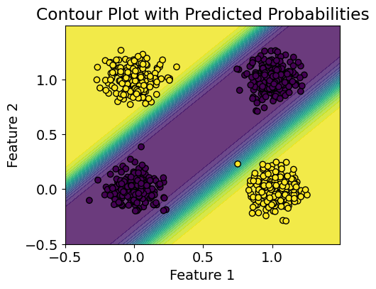
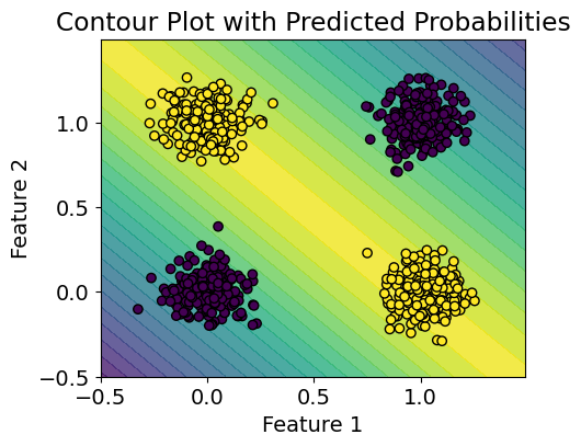
# visualize the classifier 

plt.rcParams.update({'font.size': 14, "figure.figsize": (5,4)})
# Create a mesh grid for the entire feature space
x_min, x_max = -0.5, 1.5
y_min, y_max = -0.5, 1.5
step = 0.01
xx, yy = np.meshgrid(np.arange(x_min, x_max, step), 
                     np.arange(y_min, y_max, step))

# Flatten the meshgrid and make predictions
mesh_input = np.c_[xx.ravel(), yy.ravel()]
predictions = model.predict(mesh_input, batch_size=len(mesh_input))

# Reshape predictions to the shape of the meshgrid
predictions = predictions.reshape(xx.shape)

# Create a contour plot
plt.contourf(xx, yy, predictions, cmap='viridis', levels=20, alpha=0.8)

# Scatter plot of the synthetic data points
plt.scatter(X[:, 0], X[:, 1], c=y, cmap='viridis', edgecolors='k')

plt.title('Contour Plot with Predicted Probabilities')
plt.xlabel('Feature 1')
plt.ylabel('Feature 2')
plt.show()

1/1 ━━━━━━━━━━━━━━━━━━━━ 0s 25ms/step

../_images/ebd968823916cac15b5e73ae201edbd52098b58d02316dfc680397f839fe33f9.png

Q1: What happens if we don’t use the “sigmoid” activation function?#

When from_logits=True, the binary crossentropy loss function in Keras will internally apply the sigmoid activation function during the computation of the loss.

# Define the model
model = Sequential()

# Add the input layer and the hidden layer
model.add(Dense(units=2, activation='elu', input_dim=2))  

# Add the output layer
model.add(Dense(units=1)) # no 'sigmoid' activation 

model.compile(optimizer=tf.keras.optimizers.SGD(learning_rate=0.1), 
              loss=tf.keras.losses.BinaryCrossentropy(from_logits=True), metrics=['accuracy'])

history = model.fit(X, y, epochs=50, batch_size=8)

Epoch 1/50
100/100 ━━━━━━━━━━━━━━━━━━━━ 0s 3ms/step - accuracy: 0.5018 - loss: 0.7686
Epoch 2/50
100/100 ━━━━━━━━━━━━━━━━━━━━ 0s 3ms/step - accuracy: 0.4594 - loss: 0.6517
Epoch 3/50
100/100 ━━━━━━━━━━━━━━━━━━━━ 0s 3ms/step - accuracy: 0.5285 - loss: 0.5928
Epoch 4/50
100/100 ━━━━━━━━━━━━━━━━━━━━ 0s 3ms/step - accuracy: 0.6146 - loss: 0.4937
Epoch 5/50
100/100 ━━━━━━━━━━━━━━━━━━━━ 0s 3ms/step - accuracy: 0.9898 - loss: 0.3510
Epoch 6/50
100/100 ━━━━━━━━━━━━━━━━━━━━ 0s 3ms/step - accuracy: 0.9979 - loss: 0.2147
Epoch 7/50
100/100 ━━━━━━━━━━━━━━━━━━━━ 0s 3ms/step - accuracy: 0.9998 - loss: 0.1319
Epoch 8/50
100/100 ━━━━━━━━━━━━━━━━━━━━ 0s 2ms/step - accuracy: 0.9954 - loss: 0.0903
Epoch 9/50
100/100 ━━━━━━━━━━━━━━━━━━━━ 0s 2ms/step - accuracy: 0.9975 - loss: 0.0638
Epoch 10/50
100/100 ━━━━━━━━━━━━━━━━━━━━ 0s 3ms/step - accuracy: 0.9981 - loss: 0.0516
Epoch 11/50
100/100 ━━━━━━━━━━━━━━━━━━━━ 0s 2ms/step - accuracy: 1.0000 - loss: 0.0385
Epoch 12/50
100/100 ━━━━━━━━━━━━━━━━━━━━ 0s 2ms/step - accuracy: 1.0000 - loss: 0.0339
Epoch 13/50
100/100 ━━━━━━━━━━━━━━━━━━━━ 0s 2ms/step - accuracy: 1.0000 - loss: 0.0306
Epoch 14/50
100/100 ━━━━━━━━━━━━━━━━━━━━ 0s 3ms/step - accuracy: 1.0000 - loss: 0.0257
Epoch 15/50
100/100 ━━━━━━━━━━━━━━━━━━━━ 0s 3ms/step - accuracy: 1.0000 - loss: 0.0232
Epoch 16/50
100/100 ━━━━━━━━━━━━━━━━━━━━ 0s 3ms/step - accuracy: 1.0000 - loss: 0.0218
Epoch 17/50
100/100 ━━━━━━━━━━━━━━━━━━━━ 0s 3ms/step - accuracy: 1.0000 - loss: 0.0191
Epoch 18/50
100/100 ━━━━━━━━━━━━━━━━━━━━ 0s 2ms/step - accuracy: 1.0000 - loss: 0.0177
Epoch 19/50
100/100 ━━━━━━━━━━━━━━━━━━━━ 0s 3ms/step - accuracy: 1.0000 - loss: 0.0158
Epoch 20/50
100/100 ━━━━━━━━━━━━━━━━━━━━ 0s 2ms/step - accuracy: 1.0000 - loss: 0.0142
Epoch 21/50
100/100 ━━━━━━━━━━━━━━━━━━━━ 0s 2ms/step - accuracy: 1.0000 - loss: 0.0172
Epoch 22/50
100/100 ━━━━━━━━━━━━━━━━━━━━ 0s 3ms/step - accuracy: 1.0000 - loss: 0.0126
Epoch 23/50
100/100 ━━━━━━━━━━━━━━━━━━━━ 0s 3ms/step - accuracy: 1.0000 - loss: 0.0105
Epoch 24/50
100/100 ━━━━━━━━━━━━━━━━━━━━ 0s 3ms/step - accuracy: 1.0000 - loss: 0.0111
Epoch 25/50
100/100 ━━━━━━━━━━━━━━━━━━━━ 0s 2ms/step - accuracy: 1.0000 - loss: 0.0119
Epoch 26/50
100/100 ━━━━━━━━━━━━━━━━━━━━ 0s 3ms/step - accuracy: 1.0000 - loss: 0.0118
Epoch 27/50
100/100 ━━━━━━━━━━━━━━━━━━━━ 0s 2ms/step - accuracy: 1.0000 - loss: 0.0100
Epoch 28/50
100/100 ━━━━━━━━━━━━━━━━━━━━ 0s 3ms/step - accuracy: 1.0000 - loss: 0.0100
Epoch 29/50
100/100 ━━━━━━━━━━━━━━━━━━━━ 0s 3ms/step - accuracy: 1.0000 - loss: 0.0074
Epoch 30/50
100/100 ━━━━━━━━━━━━━━━━━━━━ 0s 3ms/step - accuracy: 1.0000 - loss: 0.0090
Epoch 31/50
100/100 ━━━━━━━━━━━━━━━━━━━━ 0s 3ms/step - accuracy: 1.0000 - loss: 0.0074
Epoch 32/50
100/100 ━━━━━━━━━━━━━━━━━━━━ 0s 2ms/step - accuracy: 1.0000 - loss: 0.0084
Epoch 33/50
100/100 ━━━━━━━━━━━━━━━━━━━━ 0s 3ms/step - accuracy: 1.0000 - loss: 0.0066
Epoch 34/50
100/100 ━━━━━━━━━━━━━━━━━━━━ 0s 2ms/step - accuracy: 1.0000 - loss: 0.0081
Epoch 35/50
100/100 ━━━━━━━━━━━━━━━━━━━━ 0s 3ms/step - accuracy: 1.0000 - loss: 0.0071
Epoch 36/50
100/100 ━━━━━━━━━━━━━━━━━━━━ 0s 3ms/step - accuracy: 1.0000 - loss: 0.0054
Epoch 37/50
100/100 ━━━━━━━━━━━━━━━━━━━━ 0s 3ms/step - accuracy: 1.0000 - loss: 0.0071
Epoch 38/50
100/100 ━━━━━━━━━━━━━━━━━━━━ 0s 3ms/step - accuracy: 1.0000 - loss: 0.0070
Epoch 39/50
100/100 ━━━━━━━━━━━━━━━━━━━━ 0s 3ms/step - accuracy: 1.0000 - loss: 0.0059
Epoch 40/50
100/100 ━━━━━━━━━━━━━━━━━━━━ 0s 3ms/step - accuracy: 1.0000 - loss: 0.0061
Epoch 41/50
100/100 ━━━━━━━━━━━━━━━━━━━━ 0s 3ms/step - accuracy: 1.0000 - loss: 0.0059
Epoch 42/50
100/100 ━━━━━━━━━━━━━━━━━━━━ 0s 3ms/step - accuracy: 1.0000 - loss: 0.0080
Epoch 43/50
100/100 ━━━━━━━━━━━━━━━━━━━━ 0s 3ms/step - accuracy: 1.0000 - loss: 0.0061
Epoch 44/50
100/100 ━━━━━━━━━━━━━━━━━━━━ 0s 3ms/step - accuracy: 1.0000 - loss: 0.0046
Epoch 45/50
100/100 ━━━━━━━━━━━━━━━━━━━━ 0s 3ms/step - accuracy: 1.0000 - loss: 0.0053
Epoch 46/50
100/100 ━━━━━━━━━━━━━━━━━━━━ 0s 3ms/step - accuracy: 1.0000 - loss: 0.0045
Epoch 47/50
100/100 ━━━━━━━━━━━━━━━━━━━━ 0s 2ms/step - accuracy: 1.0000 - loss: 0.0073
Epoch 48/50
100/100 ━━━━━━━━━━━━━━━━━━━━ 0s 3ms/step - accuracy: 1.0000 - loss: 0.0044
Epoch 49/50
100/100 ━━━━━━━━━━━━━━━━━━━━ 0s 2ms/step - accuracy: 1.0000 - loss: 0.0044
Epoch 50/50
100/100 ━━━━━━━━━━━━━━━━━━━━ 0s 3ms/step - accuracy: 1.0000 - loss: 0.0045

# visualize the classifier 

plt.rcParams.update({'font.size': 14, "figure.figsize": (5,4)})
# Create a mesh grid for the entire feature space
x_min, x_max = -0.5, 1.5
y_min, y_max = -0.5, 1.5
step = 0.01
xx, yy = np.meshgrid(np.arange(x_min, x_max, step), 
                     np.arange(y_min, y_max, step))

# Flatten the meshgrid and make predictions
mesh_input = np.c_[xx.ravel(), yy.ravel()]
predictions = model.predict(mesh_input, batch_size=len(mesh_input))

# Reshape predictions to the shape of the meshgrid
predictions = predictions.reshape(xx.shape)

# Create a contour plot
plt.contourf(xx, yy, predictions, cmap='viridis', levels=20, alpha=0.8)

# Scatter plot of the synthetic data points
plt.scatter(X[:, 0], X[:, 1], c=y, cmap='viridis', edgecolors='k')

plt.title('Contour Plot with Predicted Probabilities')
plt.xlabel('Feature 1')
plt.ylabel('Feature 2')
plt.show()

1/1 ━━━━━━━━━━━━━━━━━━━━ 0s 19ms/step

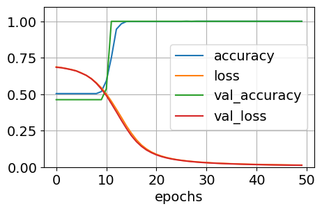
../_images/b7ceb2dd7ea27abed23cdd393eaf6e135e7719a53b46f4a655918e0a6c669160.png

Q2: How to set aside validation data?#

# Define the model
model = Sequential()

# Add the input layer and the hidden layer
model.add(Dense(units=2, activation='elu', input_dim=2))  

# Add the output layer
model.add(Dense(units=1)) # no 'sigmoid' activation 

model.compile(optimizer=tf.keras.optimizers.SGD(learning_rate=0.1), 
              loss=tf.keras.losses.BinaryCrossentropy(from_logits=True), metrics=['accuracy'])

history = model.fit(X, y, epochs=50, batch_size=16, validation_split=0.1)

Epoch 1/50
45/45 ━━━━━━━━━━━━━━━━━━━━ 0s 5ms/step - accuracy: 0.5077 - loss: 0.6893 - val_accuracy: 0.4625 - val_loss: 0.6845
Epoch 2/50
45/45 ━━━━━━━━━━━━━━━━━━━━ 0s 3ms/step - accuracy: 0.5055 - loss: 0.6845 - val_accuracy: 0.4625 - val_loss: 0.6818
Epoch 3/50
45/45 ━━━━━━━━━━━━━━━━━━━━ 0s 3ms/step - accuracy: 0.4992 - loss: 0.6786 - val_accuracy: 0.4625 - val_loss: 0.6752
Epoch 4/50
45/45 ━━━━━━━━━━━━━━━━━━━━ 0s 3ms/step - accuracy: 0.5259 - loss: 0.6706 - val_accuracy: 0.4625 - val_loss: 0.6681
Epoch 5/50
45/45 ━━━━━━━━━━━━━━━━━━━━ 0s 3ms/step - accuracy: 0.4924 - loss: 0.6599 - val_accuracy: 0.4625 - val_loss: 0.6595
Epoch 6/50
45/45 ━━━━━━━━━━━━━━━━━━━━ 0s 3ms/step - accuracy: 0.5068 - loss: 0.6504 - val_accuracy: 0.4625 - val_loss: 0.6446
Epoch 7/50
45/45 ━━━━━━━━━━━━━━━━━━━━ 0s 3ms/step - accuracy: 0.4854 - loss: 0.6331 - val_accuracy: 0.4625 - val_loss: 0.6294
Epoch 8/50
45/45 ━━━━━━━━━━━━━━━━━━━━ 0s 3ms/step - accuracy: 0.5129 - loss: 0.6095 - val_accuracy: 0.4625 - val_loss: 0.6058
Epoch 9/50
45/45 ━━━━━━━━━━━━━━━━━━━━ 0s 3ms/step - accuracy: 0.5115 - loss: 0.5859 - val_accuracy: 0.4625 - val_loss: 0.5749
Epoch 10/50
45/45 ━━━━━━━━━━━━━━━━━━━━ 0s 3ms/step - accuracy: 0.5033 - loss: 0.5530 - val_accuracy: 0.4625 - val_loss: 0.5356
Epoch 11/50
45/45 ━━━━━━━━━━━━━━━━━━━━ 0s 3ms/step - accuracy: 0.5509 - loss: 0.5148 - val_accuracy: 0.5375 - val_loss: 0.4904
Epoch 12/50
45/45 ━━━━━━━━━━━━━━━━━━━━ 0s 3ms/step - accuracy: 0.7014 - loss: 0.4515 - val_accuracy: 1.0000 - val_loss: 0.4357
Epoch 13/50
45/45 ━━━━━━━━━━━━━━━━━━━━ 0s 3ms/step - accuracy: 0.9555 - loss: 0.4051 - val_accuracy: 1.0000 - val_loss: 0.3790
Epoch 14/50
45/45 ━━━━━━━━━━━━━━━━━━━━ 0s 3ms/step - accuracy: 0.9772 - loss: 0.3506 - val_accuracy: 1.0000 - val_loss: 0.3208
Epoch 15/50
45/45 ━━━━━━━━━━━━━━━━━━━━ 0s 3ms/step - accuracy: 0.9968 - loss: 0.3006 - val_accuracy: 1.0000 - val_loss: 0.2654
Epoch 16/50
45/45 ━━━━━━━━━━━━━━━━━━━━ 0s 3ms/step - accuracy: 0.9987 - loss: 0.2419 - val_accuracy: 1.0000 - val_loss: 0.2152
Epoch 17/50
45/45 ━━━━━━━━━━━━━━━━━━━━ 0s 3ms/step - accuracy: 0.9960 - loss: 0.1996 - val_accuracy: 1.0000 - val_loss: 0.1744
Epoch 18/50
45/45 ━━━━━━━━━━━━━━━━━━━━ 0s 3ms/step - accuracy: 0.9971 - loss: 0.1608 - val_accuracy: 1.0000 - val_loss: 0.1424
Epoch 19/50
45/45 ━━━━━━━━━━━━━━━━━━━━ 0s 3ms/step - accuracy: 0.9991 - loss: 0.1303 - val_accuracy: 1.0000 - val_loss: 0.1173
Epoch 20/50
45/45 ━━━━━━━━━━━━━━━━━━━━ 0s 3ms/step - accuracy: 0.9993 - loss: 0.1054 - val_accuracy: 1.0000 - val_loss: 0.0987
Epoch 21/50
45/45 ━━━━━━━━━━━━━━━━━━━━ 0s 3ms/step - accuracy: 0.9998 - loss: 0.0887 - val_accuracy: 1.0000 - val_loss: 0.0837
Epoch 22/50
45/45 ━━━━━━━━━━━━━━━━━━━━ 0s 3ms/step - accuracy: 0.9997 - loss: 0.0782 - val_accuracy: 1.0000 - val_loss: 0.0722
Epoch 23/50
45/45 ━━━━━━━━━━━━━━━━━━━━ 0s 3ms/step - accuracy: 0.9940 - loss: 0.0701 - val_accuracy: 1.0000 - val_loss: 0.0631
Epoch 24/50
45/45 ━━━━━━━━━━━━━━━━━━━━ 0s 3ms/step - accuracy: 0.9984 - loss: 0.0600 - val_accuracy: 1.0000 - val_loss: 0.0557
Epoch 25/50
45/45 ━━━━━━━━━━━━━━━━━━━━ 0s 3ms/step - accuracy: 0.9999 - loss: 0.0521 - val_accuracy: 1.0000 - val_loss: 0.0501
Epoch 26/50
45/45 ━━━━━━━━━━━━━━━━━━━━ 0s 3ms/step - accuracy: 0.9971 - loss: 0.0466 - val_accuracy: 1.0000 - val_loss: 0.0454
Epoch 27/50
45/45 ━━━━━━━━━━━━━━━━━━━━ 0s 3ms/step - accuracy: 1.0000 - loss: 0.0414 - val_accuracy: 1.0000 - val_loss: 0.0410
Epoch 28/50
45/45 ━━━━━━━━━━━━━━━━━━━━ 0s 3ms/step - accuracy: 0.9993 - loss: 0.0358 - val_accuracy: 1.0000 - val_loss: 0.0377
Epoch 29/50
45/45 ━━━━━━━━━━━━━━━━━━━━ 0s 3ms/step - accuracy: 1.0000 - loss: 0.0353 - val_accuracy: 1.0000 - val_loss: 0.0345
Epoch 30/50
45/45 ━━━━━━━━━━━━━━━━━━━━ 0s 3ms/step - accuracy: 1.0000 - loss: 0.0335 - val_accuracy: 1.0000 - val_loss: 0.0319
Epoch 31/50
45/45 ━━━━━━━━━━━━━━━━━━━━ 0s 3ms/step - accuracy: 1.0000 - loss: 0.0319 - val_accuracy: 1.0000 - val_loss: 0.0299
Epoch 32/50
45/45 ━━━━━━━━━━━━━━━━━━━━ 0s 3ms/step - accuracy: 1.0000 - loss: 0.0315 - val_accuracy: 1.0000 - val_loss: 0.0277
Epoch 33/50
45/45 ━━━━━━━━━━━━━━━━━━━━ 0s 3ms/step - accuracy: 1.0000 - loss: 0.0304 - val_accuracy: 1.0000 - val_loss: 0.0261
Epoch 34/50
45/45 ━━━━━━━━━━━━━━━━━━━━ 0s 3ms/step - accuracy: 1.0000 - loss: 0.0246 - val_accuracy: 1.0000 - val_loss: 0.0246
Epoch 35/50
45/45 ━━━━━━━━━━━━━━━━━━━━ 0s 3ms/step - accuracy: 1.0000 - loss: 0.0250 - val_accuracy: 1.0000 - val_loss: 0.0232
Epoch 36/50
45/45 ━━━━━━━━━━━━━━━━━━━━ 0s 3ms/step - accuracy: 1.0000 - loss: 0.0221 - val_accuracy: 1.0000 - val_loss: 0.0218
Epoch 37/50
45/45 ━━━━━━━━━━━━━━━━━━━━ 0s 3ms/step - accuracy: 1.0000 - loss: 0.0216 - val_accuracy: 1.0000 - val_loss: 0.0209
Epoch 38/50
45/45 ━━━━━━━━━━━━━━━━━━━━ 0s 3ms/step - accuracy: 1.0000 - loss: 0.0233 - val_accuracy: 1.0000 - val_loss: 0.0197
Epoch 39/50
45/45 ━━━━━━━━━━━━━━━━━━━━ 0s 3ms/step - accuracy: 1.0000 - loss: 0.0220 - val_accuracy: 1.0000 - val_loss: 0.0189
Epoch 40/50
45/45 ━━━━━━━━━━━━━━━━━━━━ 0s 3ms/step - accuracy: 1.0000 - loss: 0.0179 - val_accuracy: 1.0000 - val_loss: 0.0178
Epoch 41/50
45/45 ━━━━━━━━━━━━━━━━━━━━ 0s 3ms/step - accuracy: 1.0000 - loss: 0.0195 - val_accuracy: 1.0000 - val_loss: 0.0171
Epoch 42/50
45/45 ━━━━━━━━━━━━━━━━━━━━ 0s 3ms/step - accuracy: 1.0000 - loss: 0.0172 - val_accuracy: 1.0000 - val_loss: 0.0163
Epoch 43/50
45/45 ━━━━━━━━━━━━━━━━━━━━ 0s 3ms/step - accuracy: 1.0000 - loss: 0.0188 - val_accuracy: 1.0000 - val_loss: 0.0157
Epoch 44/50
45/45 ━━━━━━━━━━━━━━━━━━━━ 0s 3ms/step - accuracy: 1.0000 - loss: 0.0146 - val_accuracy: 1.0000 - val_loss: 0.0150
Epoch 45/50
45/45 ━━━━━━━━━━━━━━━━━━━━ 0s 3ms/step - accuracy: 1.0000 - loss: 0.0164 - val_accuracy: 1.0000 - val_loss: 0.0146
Epoch 46/50
45/45 ━━━━━━━━━━━━━━━━━━━━ 0s 3ms/step - accuracy: 1.0000 - loss: 0.0174 - val_accuracy: 1.0000 - val_loss: 0.0141
Epoch 47/50
45/45 ━━━━━━━━━━━━━━━━━━━━ 0s 3ms/step - accuracy: 1.0000 - loss: 0.0147 - val_accuracy: 1.0000 - val_loss: 0.0134
Epoch 48/50
45/45 ━━━━━━━━━━━━━━━━━━━━ 0s 3ms/step - accuracy: 1.0000 - loss: 0.0150 - val_accuracy: 1.0000 - val_loss: 0.0129
Epoch 49/50
45/45 ━━━━━━━━━━━━━━━━━━━━ 0s 3ms/step - accuracy: 1.0000 - loss: 0.0156 - val_accuracy: 1.0000 - val_loss: 0.0127
Epoch 50/50
45/45 ━━━━━━━━━━━━━━━━━━━━ 0s 3ms/step - accuracy: 1.0000 - loss: 0.0146 - val_accuracy: 1.0000 - val_loss: 0.0122

history.history.keys()

dict_keys(['accuracy', 'loss', 'val_accuracy', 'val_loss'])

pd.DataFrame(history.history).plot(figsize=(5, 3))
plt.grid(True)
plt.gca().set_ylim(0, 1.1)
plt.xlabel('epochs')
plt.show()

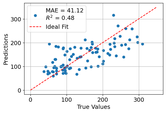
../_images/816b1417d06f5bb56140ccca0f03429023ebc2cfde6449bc29934e6c577ce436.png

In this example, we build and train a multilayer perceptron (MLP) regressor using Keras to predict disease progression based on the Diabetes dataset from Scikit-learn.
The model uses three hidden layers with ReLU activation functions and incorporates Dropout regularization to prevent overfitting.
The input features are first standardized to improve training stability and performance.
We train the model using the Adam optimizer and mean squared error (MSE) loss, and evaluate its performance using the mean absolute error (MAE) and coefficient of determination (R² score).
A final scatter plot compares the model’s predictions to the true target values, offering a visual assessment of the model’s accuracy.

# Import libraries
import numpy as np
import matplotlib.pyplot as plt
from sklearn.datasets import load_diabetes
from sklearn.model_selection import train_test_split
from sklearn.preprocessing import StandardScaler
from sklearn.metrics import mean_absolute_error, r2_score

import tensorflow as tf
from tensorflow import keras
from tensorflow.keras import layers

# Load the diabetes dataset
diabetes = load_diabetes()
X, y = diabetes.data, diabetes.target

# Split into training and testing sets
X_train, X_test, y_train, y_test = train_test_split(
    X, y, test_size=0.2, random_state=42
)

# Standardize the features
scaler = StandardScaler()
X_train_scaled = scaler.fit_transform(X_train)
X_test_scaled = scaler.transform(X_test)

# Build an improved MLP model with dropout only
model = keras.Sequential([
    layers.Input(shape=(X.shape[1],)),
    layers.Dense(128, activation='relu'),
    layers.Dropout(0.2),
    
    layers.Dense(64, activation='relu'),
    layers.Dropout(0.2),
    
    layers.Dense(32, activation='relu'),
    layers.Dense(1)  # Output layer for regression
])

# Compile the model
model.compile(optimizer='adam', loss='mse', metrics=['mae'])

# Train the model
history = model.fit(
    X_train_scaled, y_train,
    epochs=150,
    batch_size=32,
    validation_split=0.1,
    verbose=0  # Change to 1 to see training progress
)

# Predict on the test set
y_pred = model.predict(X_test_scaled).flatten()

# Compute metrics
mae = mean_absolute_error(y_test, y_pred)
r2 = r2_score(y_test, y_pred)

# Plot predictions vs. true values
plt.figure(figsize=(6, 4))
plt.scatter(y_test, y_pred, label=f"MAE = {mae:.2f}\n$R^2$ = {r2:.2f}")
plt.plot([0, 350], [0, 350], 'r--', label="Ideal Fit")
plt.xlabel("True Values")
plt.ylabel("Predictions")
plt.legend(loc="upper left")
plt.grid(True)
plt.show()

3/3 ━━━━━━━━━━━━━━━━━━━━ 0s 13ms/step

../_images/39e70cda0fb2fff338ba26c8cc841331c6788010512ad3d855b5c88fbe8d909d.png