The Machine Learning Landscape

The Machine Learning Landscape#

Machine Learning Methods#

Module 1: The Machine Learning Landscape#

Instructor: Farhad Pourkamali#

Overview#

Definition of Machine Learning (https://youtu.be/ZvV0XTMlpJg)
Components and Types of Machine Learning (https://youtu.be/VWSf9yjEseQ)
- Components of Machine Learning:
  - Data
  - Models
  - Training
  - Evaluation
- Categorization Based on Data Supervision:
  - Supervised Learning
  - Unsupervised Learning
  - Semi-Supervised Learning
- Categorization Based on Learning Strategy:
  - Model-Based Learning
  - Instance-Based Learning
Mathematical Concepts Behind Machine Learning (https://youtu.be/fjWMBNU_Z0Y)
- Probability and statistics, linear algebra, optimization
Programming Concepts for Machine Learning (https://youtu.be/8aeGfeDNH3E)
- Python Basics
  - Variables, loops, conditional statements, and functions
- Object-Oriented Programming (OOP)
  - Classes: Blueprints for creating objects
  - Objects: Instances of classes
  - Attributes: Variables that store data within an object
  - Methods: Define behaviors of an object
- NumPy: https://numpy.org/doc/stable/index.html#
  - Core library for numerical computations
  - Efficient array manipulations
- Pandas: https://pandas.pydata.org/docs/index.html
  - Data manipulation and analysis
  - Handling datasets and missing values

1. Definition of Machine Learning#

Why Use Machine Learning?#

Let’s design a spam filtering system using traditional programming techniques
- Manually write rules to detect spam emails
- For example, look for specific keywords or phrases, such as “credit card” or “account number,” and flag emails containing these words as spam
- Requires a long list of complex rules that need constant updates as spammers adapt
A spam filter based on machine learning aims to automatically learn which words and phrases are good predictors or inputs
- The filter uses a supervised learning approach, where it is trained on a data set of labeled examples: emails marked as “spam” or “not spam”
- The model identifies patterns in the training data that predict the label
- No need to manually update rules
- Can learn and adjust as new types of spam emerge
- Learns subtle patterns and relationships in the data that humans may miss

What Is Machine Learning?#

Tom Mitchell’s definition of machine learning (https://www.cs.cmu.edu/~tom/):

A computer program is said to learn from experience E with respect to some class of tasks T and performance measure P, if its performance at tasks in T, as measured by P, improves with experience E.
Application to spam email detection:
- Experience (E): The data set comprising emails labeled as “spam” or “not spam.” This labeled data serves as the training set, enabling the model to learn distinguishing features of spam emails.
- Task (T): Classifying incoming emails as either “spam” or “not spam.” This involves analyzing email content and metadata to make accurate classifications.
- Performance Measure (P): The accuracy of the email classifications, defined as the proportion of correctly identified emails (both spam and not spam) out of the total number of emails processed. Higher accuracy indicates better model performance.
Farhad Pourkamali’s definition of machine learning:

Machine learning can be conceptualized as a teacher-student framework, where the teacher provides examples, training data, or feedback. The student, represented by the machine learning model, aims to learn patterns from this input and apply that knowledge to provide answers to new problems.

2. Components and Types of Machine Learning#

Components of Machine Learning#

Data
- The information used to teach and train the machine learning system, representing the raw material from which patterns and insights are derived.
- Examples include text, images, or numerical data sets.
Models
- Abstract algorithmic structures or mathematical representations designed to learn from data.
- Models do not inherently “know” or “learn” anything until trained. They provide a framework or set of rules (guidelines) to capture underlying patterns and relationships in the data.
Training
- The process of exposing the model to data, allowing it to adjust its internal parameters and learn relationships
Evaluation
- A systematic method of assessing the model’s performance on unseen data.
- Evaluation helps identify areas for potential improvement.

Types of Machine Learning#

Machine learning models can be categorized based on the level of supervision they receive during training. The level of supervision refers to the amount and type of labeled data to learn from.
- Supervised Learning
  - Definition: Learning from labeled data sets where the input-output pairs are known, enabling the model to make predictions or classifications.
  - Applications: Used in tasks like email spam detection and handwriting recognition.
- Unsupervised Learning
  - Definition: Learning from unlabeled data to identify inherent structures or patterns without predefined labels.
  - Applications: Employed in clustering customers based on purchasing behavior and reducing data dimensionality.
  - Generative models often fall under unsupervised learning as they learn patterns in data without explicit labels, used for image generation, text synthesis, or audio creation.
- Semi-Supervised Learning
  - Definition: Combines a small amount of labeled data with a large amount of unlabeled data during training, bridging supervised and unsupervised learning.
  - Applications: In many real-world cases, we have a limited budget for labeling new samples, as manually labeling data can be costly or resource-intensive.
    - Semi-supervised learning makes efficient use of this budget by extracting as much information as possible from unlabeled data while relying on minimal labeled examples.

Supervised Learning (Making Predictions)#

Supervised learning can be divided into two main types based on the nature of the label:
- Regression: Predicts a continuous output variable (e.g., a real number).
- Classification: Predicts a discrete output variable (e.g., a category or class label).
The difference in target types directly impacts:
- The way models process data.
- How they output predictions.
- How error is measured during training.
When dealing with categorical targets, there is no obvious notion of distance between classes.

Model-Based vs Instance-Based Learning#

Machine learning models can be categorized based on their learning strategies, notably into model-based and instance-based approaches.
- Model-based learning:
  - Emphasizes learning a fixed set of parameters or rules during the training stage to make predictions.
  - Once trained, the model’s parameters remain fixed, and predictions are made using this generalized model.
- Instance-based learning
  - Memorizes the training data and makes predictions for new instances by comparing them to stored examples (e.g., k-Nearest Neighbors and Radial Basis Function networks).
  - Does not explicitly build a generalized model but relies on the similarity between instances.
As a result, model-based approaches generally have faster prediction times but slower training.

3. Mathematical Concepts Behind Machine Learning#

Notation#

Supervised learning: learn a mapping or function \(f\) from inputs (features/predictors) \(\mathbf{x}\in\mathcal{X}\) to outputs \(\mathbf{y}\in\mathcal{Y}\). The data set is given in the form of \(N\) input-output pairs \(\mathcal{D}=\{(\mathbf{x}_n,\mathbf{y}_n)\}_{n=1}^N\)
- \(N\) is the sample size and the number of features is \(D\), i.e., \(\mathcal{X}=\mathbb{R}^D\)
- Multi-class classification: \(\mathcal{Y}=\{1,2,\ldots, C\}\)
- If we have two classes only (binary classification):
  - \(\mathcal{Y}=\{0,1\}\)
  - \(\mathcal{Y}=\{-1,1\}\)
- We often make an assumption about the functional form or shape of \(f\)

Empirical Risk Minimization#

Joint Distribution and Population Risk

In machine learning, we assume there is an underlying joint probability distribution \(P_{XY}\) over the input \(\mathbf{x} \in \mathcal{X}\) and output \(y \in \mathcal{Y}\).
The goal is to find a model \(f(\mathbf{x}; \boldsymbol{\theta})\) parameterized by \(\boldsymbol{\theta}\) that minimizes the expected error, or population risk, defined as:

\[ R(\boldsymbol{\theta}) := \mathbb{E}_{(\mathbf{x},y)\sim P_{XY}}[l(y, f(\mathbf{x}; \boldsymbol{\theta}))] \]

where \(l(y, f(\mathbf{x}; \boldsymbol{\theta}))\) is the loss function measuring the discrepancy between the true label \(y\) and the model’s prediction \(f(\mathbf{x}; \boldsymbol{\theta})\).

Sampling and Empirical Risk

Since the true distribution \(P_{XY}\) is unknown, we rely on a data set of \(N\) i.i.d. samples \(\{(\mathbf{x}_n, y_n)\}_{n=1}^N\) drawn from \(P_{XY}\). Using this data set, we compute the empirical risk, which serves as an approximation of the population risk:

\[ \mathcal{L}(\boldsymbol{\theta}) := \frac{1}{N} \sum_{n=1}^N l(y_n, f(\mathbf{x}_n; \boldsymbol{\theta})) \]

Empirical Risk Minimization

The objective of Empirical Risk Minimization (ERM) is to find the parameters \(\boldsymbol{\theta}\) that minimize the empirical risk:

\[ {\boldsymbol{\theta}}^* := \arg\min_{\boldsymbol{\theta}} \mathcal{L}(\boldsymbol{\theta}) \]

By solving this optimization problem, we identify the model that best fits the training data.

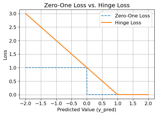
Example: Zero-One Loss for Classification Problems#

The zero-one loss is a simple loss function defined as:

\[ l(y, \hat{y}) = I(y \neq \hat{y}) \]

where \(I(y \neq \hat{y})\) is an indicator function:

\[\begin{split} I(y \neq \hat{y}) = \begin{cases} 1 & \text{if } y \neq \hat{y} \\ 0 & \text{if } y = \hat{y} \end{cases} \end{split}\]

Using the zero-one loss, the empirical risk becomes the misclassification rate:

\[ \mathcal{L}(\boldsymbol{\theta}) = \frac{1}{N} \sum_{n=1}^N I(y_n \neq f(\mathbf{x}_n; \boldsymbol{\theta})) \]

Example: Hinge Loss (For Classification with Margin)#

The hinge loss is commonly used in classification problems, particularly with support vector machines (SVMs). It is defined as:

\[ l(y, \hat{y}) = \max(0, 1 - y \cdot \hat{y}) \]

where:

\(y \in \{-1, +1\}\) represents the true label.
\(\hat{y} = f(\mathbf{x}; \boldsymbol{\theta})\) is the predicted score or margin.

The hinge loss penalizes predictions that are incorrect or fall within the margin:

If \(y \cdot \hat{y} \geq 1\): The loss is zero, meaning the prediction is correct and beyond the margin.
If \(y \cdot \hat{y} < 1\): The loss increases linearly as the prediction deviates from the correct classification boundary.

In simple terms, the hinge loss encourages predictions to be not just correct, but confidently correct by maximizing the margin between classes.

Python Experiment#

In the following, we assume the labels are binary: \(y\in\{-1,+1\}\)
We assume that the predicted value \(\hat{y}\) is a continuous score, and its sign determines the predicted class
- Positive sign (\(\hat{y}>0\)): Predicted class is +1
- Negative sign (\(\hat{y}<0\)): Predicted class is -1
Zero-One Loss: Evaluates whether the sign of \(\hat{y}\) matches the true label \(y\) (here \(y\) is +1)
Hinge loss provides smoother feedback compared to the zero-one loss.

import numpy as np
import matplotlib.pyplot as plt

plt.rcParams.update({'font.size': 12, "figure.figsize": (6,4)})

# Define zero-one loss
def zero_one_loss(y_true, y_pred):
    return np.where(y_true * y_pred < 0, 1, 0)

# Define hinge loss
def hinge_loss(y_true, y_pred):
    return np.maximum(0, 1 - y_true * y_pred)

# Generate a range of predicted values (y_pred)
y_pred = np.linspace(-2, 2, 500)

# Set the true label (y_true = 1 or -1)
y_true = 1

# Calculate losses
zero_one = zero_one_loss(y_true, y_pred)
hinge = hinge_loss(y_true, y_pred)

# Plot the losses
plt.plot(y_pred, zero_one, label="Zero-One Loss", linestyle="--")
plt.plot(y_pred, hinge, label="Hinge Loss", linewidth=2)
plt.title("Zero-One Loss vs. Hinge Loss")
plt.xlabel("Predicted Value (y_pred)")
plt.ylabel("Loss")
plt.legend()
plt.grid(True)
plt.show()

../_images/29186d9219ae281a1bea974bbd87aacb3bce1ae4902a7eecc2d5b94af5a7097e.png

General Workflow for Machine Learning Models#

Data is fed into the model to pass through layer(s), each applying transformations to extract useful patterns or representations (linear algebra)
The loss function computes the difference between predicted and expected outputs, quantifying prediction errors (probability and statistics)
We adjust the parameters (iteratively) to minimize the loss function (optimization)

Generalization#

Divide the data into training and test sets: \(\mathcal{D}_{\text{train}}\) and \(\mathcal{D}_{\text{test}}\)

Train your model using the training set and test it using the test set
Training risk: \(\mathcal{L}_{\text{train}}:=\frac{1}{|\mathcal{D}_{\text{train}}|}\sum_{(\mathbf{x},y)\in\mathcal{D}_{\text{train}}}l(y,f(\mathbf{x};\boldsymbol{\theta}))\)
Test risk: \(\mathcal{L}_{\text{test}}:=\frac{1}{|\mathcal{D}_{\text{test}}|}\sum_{(\mathbf{x},y)\in\mathcal{D}_{\text{test}}}l(y,f(\mathbf{x};\boldsymbol{\theta}))\)
Overfitting happens when \(\mathcal{L}_{\text{test}}\gg \mathcal{L}_{\text{train}}\)

4. Programming Concepts for Machine Learning#

A list in Python is a versatile, ordered collection of elements (which can be of different data types) that is mutable, allowing elements to be added, removed, or modified

#  List 

alist = [1, "a" , 5 , 5.3]

print(alist, '\n', len(alist), '\n', alist[2], '\n', alist[-1])

[1, 'a', 5, 5.3] 


3

A tuple in Python is an ordered, immutable collection of elements (which can be of different data types) that cannot be changed after creation

# Tuples are just like lists with the exception that 
# tuples cannot be changed once declared

t = (1, "a", "string", 1+2)

print(t, '\t', type(t))

print(t[1])

(1, 'a', 'string', 3) 	 <class 'tuple'>
a

A dictionary in Python is an unordered, mutable collection of key-value pairs, where each key is unique and used to efficiently access its corresponding value

# Dictionary holds key:value pairs
# indexing is done with the help of keys

d = {}

d["fall"] = 50 

d["spring"] = 80

# print(d)

print(d["fall"])

type(d)

dict

A for loop in Python is used to iterate over a sequence (like a list, tuple, or string) or other iterable objects, executing a block of code for each element in the sequence

# for loop 

alist = [1, 3, 5, 7, 9]

# Method 1

for item in alist:
    
    print(item)

The len() function returns the total number of elements in the list
The range() function generates a sequence of numbers starting from 0 (default) up to, but not including, len(alist)

for index in range(len(alist)):
    print(index)

# Method 2 

for index in range(len(alist)):
    
    print(alist[index])

if, elif, and else in Python are conditional statements used to execute specific blocks of code based on whether a condition is true (if), test additional conditions (elif), or provide a fallback when all conditions are false (else)

# if statement

x = 5

if x < 0:
    print('Negative')
elif x == 0:
    print('Zero')
else:
    print('Positive')

Positive

A function in Python is a reusable block of code that performs a specific task, defined using the def keyword, and can accept inputs (parameters), execute operations, and optionally return a value

# defining functions 

def square(num):
    num_new = num ** 2
    return num_new

print(square(4))

def square(num):
    '''
    Calculate a number raise to the power of 2.   
    '''
    # this is comment 
    num_new = num ** 2
    return num_new

# More than one output 

def square_cube(num):
    '''
    Calculate a number raise to the power of 2
    Calculate a number raise to the power of 3
    '''
    num_new1 = num ** 2
    num_new2 = num ** 3
    return num_new1, num_new2

result = square_cube(3)

print(result, type(result))

(9, 27) <class 'tuple'>

Object-Oriented programming (OOP)#

Ideal for building versatile and reusable tools/frameworks
Code as a collection and interaction of objects
Object: a data structure incorporating information about
- State: How the object looks or what properties it has
- Behavior: What the object does or how to operate on
  - Python: State –> Attribute (variable), Behavior –> Method (function)
Class: Blueprint or template for objects outlining possible states and behaviors

To explain OOP, let us consider the simple case of linear regression with one input feature, that is \(f(x;\beta_0,\beta_1) = \beta_0 + \beta_1 x\). Given a set of input-output pairs \((x_1, y_1), \ldots, (x_N, y_N)\), this is how you can find the intercept and slope: (Equation 3.4 of An Introduction to Statistical Learning with Applications in Python or ISL: https://www.statlearning.com/)

\[ \beta_1^* = \frac{\sum_{n=1}^N (x_n - \bar{x})(y_n - \bar{y})}{\sum_{n=1}^N (x_n - \bar{x})^2} \]

and

\[ \beta_0^* = \bar{y} - \beta_1^* \bar{x} \]

where \(\bar{x}\) and \(\bar{y}\) are sample means.

class SimpleLinearRegression:
    
    def __init__(self):
        # Initialize parameters (beta_0 and beta_1) to None
        self.beta_0 = None
        self.beta_1 = None

    def fit(self, x, y):
        """
        Fit the model to the data using the provided formulas.
        Args:
        x: List or array of input features
        y: List or array of target values
        """
        n = len(x)
        x_mean = sum(x) / n
        y_mean = sum(y) / n

        # Calculate beta_1 using the provided formula
        numerator = sum((xi - x_mean) * (yi - y_mean) for xi, yi in zip(x, y))
        denominator = sum((xi - x_mean) ** 2 for xi in x)
        self.beta_1 = numerator / denominator

        # Calculate beta_0 using the provided formula
        self.beta_0 = y_mean - self.beta_1 * x_mean

    def predict(self, x):
        """
        Predict the target values for given input features.
        Args:
        x: List or array of input features
        Returns:
        List of predicted values
        """
        return [self.beta_0 + self.beta_1 * xi for xi in x]


# Example usage:
x = [1, 2, 3, 4, 5]
y = [5, 8, 11, 14, 17]  # Corresponding to beta_0 = 2 and beta_1 = 3

# Create an instance of the SimpleLinearRegression class
model = SimpleLinearRegression()

# Fit the model to the data
model.fit(x, y)

# Predict values for the input x
predicted_y = model.predict([10])

# Print results
print("Learned parameters:")
print(f"Beta_0 (Intercept): {model.beta_0}")
print(f"Beta_1 (Slope): {model.beta_1}")
print("Predicted values:", predicted_y)

Learned parameters:
Beta_0 (Intercept): 2.0
Beta_1 (Slope): 3.0
Predicted values: [32.0]

NumPy#

NumPy ndarrays provide an efficient, multidimensional array structure for numerical computation, enabling fast operations on large data sets with support for advanced mathematical, logical, and statistical functions
1D (vector) and 2D arrays (matrix)

\[\begin{split}\mathbf{a}=\begin{bmatrix}a_1\\a_2\\\vdots\\a_n\end{bmatrix}\in\mathbb{R}^n,\;\mathbf{A}=\begin{bmatrix}a_{11}&\ldots&a_{1m}\\ \vdots&&\vdots\\a_{n1}&&a_{nm}\end{bmatrix}\in\mathbb{R}^{n\times m}\end{split}\]

import numpy as np 

a = np.array([1,2,3,4])

A = np.array([[1,2], [3,4]])

print(a.shape, A.shape, type(a))

(4,) (2, 2) <class 'numpy.ndarray'>

print(a)

[1 2 3 4]

print(A)

[[1 2]
 [3 4]]

a.ndim

A.ndim

array([1, 2, 3, 4])

a.reshape(2,2)

array([[1, 2],
       [3, 4]])

array([[1, 2],
       [3, 4]])

# reshape

b = A.reshape(4,)

print(b, b.shape)

[1 2 3 4] (4,)

# True if two arrays have the same shape and elements

np.array_equal(a, b)

True

# transpose a matrix by switching its rows with its columns

print(A, '\n\n', np.transpose(A))

[[1 2]
 [3 4]] 

 [[1 3]
 [2 4]]

A.T

array([[1, 3],
       [2, 4]])

x = np.array([3, 4])

from numpy import linalg # implementations of standard linear algebra algorithms

print(linalg.norm(x))

5.0

Dot product or inner product#

\[\langle\mathbf{x},\mathbf{y}\rangle=\sum_{i=1}^n x_iy_i\]

y = np.array([2,3])

np.dot(x, y)

# norm of x squared 
np.dot(x, x)

Matrix multiplication#

Method 1 \(\begin{bmatrix}a_{11} & \ldots & a_{1n}\\\vdots & & \vdots\\a_{m1}&\ldots &a_{mn}\end{bmatrix}\begin{bmatrix}x_1\\\vdots\\x_n\end{bmatrix}=x_1\begin{bmatrix}a_{11}\\\vdots\\a_{m1}\end{bmatrix}+\ldots+x_n\begin{bmatrix}a_{1n}\\\vdots\\a_{mn}\end{bmatrix}\)
Method 2 \(\begin{bmatrix}a_{11} & \ldots & a_{1n}\\\vdots & & \vdots\\a_{m1}&\ldots &a_{mn}\end{bmatrix}\begin{bmatrix}x_1\\\vdots\\x_n\end{bmatrix}=\begin{bmatrix}\sum_{i=1}^n a_{1i}x_i\\\vdots\\\sum_{i=1}^na_{mi}x_i\end{bmatrix}\)

A = np.array([[1,2,3],[4,5,6]])

x = np.array([[2],[4],[5]]) 

z = np.matmul(A,x)

print(z)

[[25]
 [58]]

Pandas#

Provides high performance, fast, easy-to-use data structures, and data analysis tools for manipulating tabular data
Dataframe
- A two dimensional data structure with columns of potentially different types

# Read CSV File into Python using Pandas
import numpy as np 
import pandas as pd


df = pd.read_csv("Credit.csv")
                 
df.head()

	Income	Limit	Rating	Cards	Age	Education	Own	Student	Married	Region	Balance
0	14.891	3606	283	2	34	11	No	No	Yes	South	333
1	106.025	6645	483	3	82	15	Yes	Yes	Yes	West	903
2	104.593	7075	514	4	71	11	No	No	No	West	580
3	148.924	9504	681	3	36	11	Yes	No	No	West	964
4	55.882	4897	357	2	68	16	No	No	Yes	South	331

len(df)

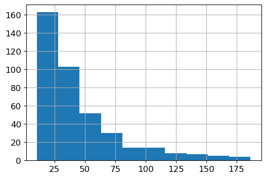
df['Income']

     14.891
    106.025
    104.593
    148.924
     55.882
        ...   
   12.096
   13.364
   57.872
   37.728
   18.701
Name: Income, Length: 400, dtype: float64

df['Income'].hist(bins=10) # in thousands of dollars

<Axes: >

../_images/36c7550f7239bc8decc9260b0f348f226725661b2cdae9fd286735df4c5b5c95.png

# select rows where the values in the Income column are less than 100
df[df['Income']<100]

	Income	Limit	Rating	Cards	Age	Education	Own	Student	Married	Region	Balance
0	14.891	3606	283	2	34	11	No	No	Yes	South	333
4	55.882	4897	357	2	68	16	No	No	Yes	South	331
5	80.180	8047	569	4	77	10	No	No	No	South	1151
6	20.996	3388	259	2	37	12	Yes	No	No	East	203
7	71.408	7114	512	2	87	9	No	No	No	West	872
...	...	...	...	...	...	...	...	...	...	...	...
395	12.096	4100	307	3	32	13	No	No	Yes	South	560
396	13.364	3838	296	5	65	17	No	No	No	East	480
397	57.872	4171	321	5	67	12	Yes	No	Yes	South	138
398	37.728	2525	192	1	44	13	No	No	Yes	South	0
399	18.701	5524	415	5	64	7	Yes	No	No	West	966

363 rows × 11 columns

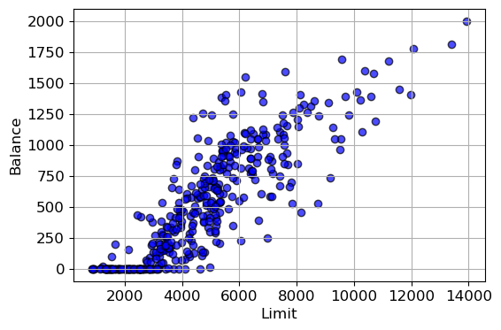
import matplotlib.pyplot as plt 

# Select two columns and convert them to lists
x_list = df['Limit'].tolist()  # Convert 'Income' column to a Python list
y_list = df['Balance'].tolist()  # Convert 'Balance' column to a Python list

# Visualize the scatter plot
plt.scatter(x_list, y_list, c='blue', alpha=0.7, edgecolors='black')
plt.xlabel('Limit')
plt.ylabel('Balance')
plt.grid(True)
plt.show()

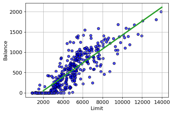
../_images/a306b027e4b00ab46d2cf47673dbcdb064e2583a123349f6a5f9fb52f28266d3.png

# Use the SimpleLinearRegression class

model = SimpleLinearRegression()

model.fit(x_list, y_list)

print(model.beta_0, model.beta_1)

-292.7904954559949 0.171637278371483

# Visualize the scatter plot and prediction line 
plt.scatter(x_list, y_list, c='blue', alpha=0.7, edgecolors='black')
plt.plot([2000, 14000], 
         [model.beta_0 + model.beta_1*2000, model.beta_0 + model.beta_1*14000],
         c = 'C2', lw=3)
plt.xlabel('Limit')
plt.ylabel('Balance')
plt.grid(True)
plt.show()

../_images/7579b96a2fb9ccce40e73f9b115035521259b2710153161e30da01ad3d63fe2a.png