Support Vector Machines#
Machine Learning Methods#
Module 6: Advanced Machine Learning Models#
Part 1: Support Vector Machines#
Instructor: Farhad Pourkamali#
Overview#
Support Vector Machines (SVMs) are supervised learning algorithms widely used for:
Classification
Regression
Key Advantages of SVMs:
Effective in high-dimensional spaces, making them ideal for complex datasets.
Still effective even when the number of features exceeds the number of samples.
Versatile, allowing the use of different kernel functions (linear, polynomial, radial basis function), with the option to define custom kernels.
Video: https://youtu.be/h6WSGd-FQL0
1. SVM Problem Formulation#
In Support Vector Machine (SVM) literature, it’s common practice to represent binary class labels as −1 and +1 (instead of 0 and 1).
This simplifies mathematical derivations and computations.
A linear SVM classifier predicts classes using the following decision rule:
The decision boundary is defined by the linear function:
Definitions:
\(\mathbf{w}\): weight vector, determines the orientation and steepness of the decision boundary.
\(b\): bias term, controls the position of the decision boundary relative to the origin.
Hyperplane:
A hyperplane is a flat subspace that separates the feature space into two distinct regions.
Examples:
In 2D, a hyperplane is a straight line.
In 3D, a hyperplane is a plane.
In higher dimensions, a hyperplane generalizes accordingly.
Sign function:
Making predictions with a linear SVM classifier:
Calculate \(f(\mathbf{x})\) and apply the sign function to determine class membership.
Training the classifier:
Training involves determining optimal \(\mathbf{w}\) and \(b\) by maximizing the margin.
Margin: the shortest distance between the hyperplane and the closest data points (support vectors) from both classes.
Maximizing this margin ensures robust, reliable predictions and better generalization to unseen data.

Finding the margin#
Step 1: Distance from a point to a hyperplane#
Consider a hyperplane defined by:
Question: How can we measure the distance of a point \(\mathbf{x}\) to this hyperplane?

Intuition:
To find the distance, project point \(\mathbf{x}\) perpendicularly onto the hyperplane.
Let’s call this projection \(\mathbf{x}^P\). Then:
where \(\mathbf{d}\) is the shortest vector from \(\mathbf{x}\) to the hyperplane.
Since \(\mathbf{d}\) is perpendicular to the hyperplane, it must be parallel to \(\mathbf{w}\):
Because the projected point \(\mathbf{x}^P\) lies exactly on the hyperplane:
Substituting the above, we get:
Solving for \(\alpha\):
Therefore, the distance from the point \(\mathbf{x}\) to the hyperplane is:
Step 2: Margin definition for dataset#
The margin is defined as the shortest distance between the hyperplane and the closest point(s) from either class:
Step 3: Finding the maximum margin hyperplane#
Our goal in training an SVM is to maximize the margin while correctly classifying all data points. This is a constrained optimization problem:
Plugging the margin definition explicitly, the optimization problem becomes:
Important note (scale invariance)#
The margin definition is scale-invariant:
Multiplying \(\mathbf{w}\) and \(b\) by a non-zero constant does not change the hyperplane.
Optimization problem#
A common choice is to fix the scale such that the distance to the nearest points (support vectors) is exactly \(1/\|\mathbf{w}\|_2\):
With this scaling convention, maximizing the margin is equivalent to minimizing the norm of the weight vector \(\mathbf{w}\):
Why is this simpler?
The condition \(y_n(\mathbf{w}^T \mathbf{x}_n + b) \geq 1\) ensures all data points are correctly classified and placed at or beyond this margin boundary.
SVM with soft constraints#
If there is no separating hyperplane, then solve
subject to constraints:
Interpretation:
\(\xi_n\) measures how much the n-th data point violates the margin constraint.
The goal is still to maximize the margin, but now we balance margin maximization against penalizing margin violations, controlled by the penalty term \(\sum_n \xi_n\).
The hyperparameter controlling this trade-off determines the balance between margin maximization and minimizing misclassification errors.
Illustration

2. Creating an SVM model using Scikit-Learn#
Documentation: https://scikit-learn.org/stable/modules/generated/sklearn.svm.SVC.html
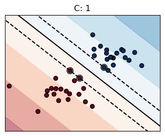
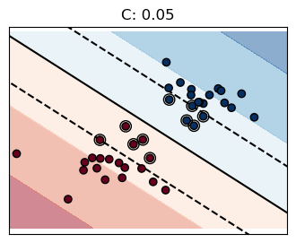
The penalty term \(C\) controls the strength of this penalty, and as a result, acts as an inverse regularization parameter
Higher \(C\) → Less regularization (tries harder to avoid margin violations, leading to a more complex decision boundary).
Lower \(C\) → More regularization (allows more margin violations, leading to a simpler decision boundary with better generalization).
The role of kernel functions:#
Linear Decision Function: In a linear SVM, the decision function is:
\[ f(\mathbf{x}) = \mathbf{w}^\top \mathbf{x} + b \]where \(\mathbf{w}\) is the weight vector, \(\mathbf{x}\) is the input feature vector, and \(b\) is the bias term.
Dual Formulation: The optimization problem can be expressed in its dual form, where the decision function depends only on the dot products between input vectors:
\[ f(\mathbf{x}) = \beta_0 +\sum_{i=1}^n \alpha_i \langle \mathbf{x},\mathbf{x}_i \rangle \]
where there are \(n\) parameters \(\alpha_i\), \(i=1,\ldots,n\), one per training observation.
Kernel Trick: To handle non-linearly separable data, we map the input features into a higher-dimensional space using a mapping function \(\varphi(\mathbf{x})\). The decision function becomes:
\[ f(\mathbf{x}) = \beta_0 +\sum_{i=1}^n \alpha_i \langle \varphi(\mathbf{x}),\varphi(\mathbf{x}_i) \rangle \]Computing \(\varphi(\mathbf{x})\) explicitly can be computationally expensive. Instead, we use a kernel function \(K(\mathbf{x}, \mathbf{x}_i)\) that computes the dot product in the higher-dimensional space without explicit mapping:
\[ K(\mathbf{x}, \mathbf{x}_i) = \langle \varphi(\mathbf{x}), \varphi(\mathbf{x}_i) \rangle \]This approach is known as the kernel trick, allowing SVMs to learn complex, non-linear decision boundaries efficiently.
Common Kernel Functions:#
Linear Kernel: \( K(\mathbf{x}_i, \mathbf{x}_j) = \mathbf{x}_i^\top \mathbf{x}_j \)
Polynomial Kernel: \( K(\mathbf{x}_i, \mathbf{x}_j) = (\mathbf{x}_i^\top \mathbf{x}_j + c)^d \)
Radial Basis Function (RBF) Kernel: \( K(\mathbf{x}_i, \mathbf{x}_j) = \exp(-\gamma \|\mathbf{x}_i - \mathbf{x}_j\|^2) \)
By choosing an appropriate kernel, SVMs can effectively handle non-linear separations in the data without explicitly transforming the feature space.
# Source: https://scikit-learn.org/stable/auto_examples/svm/plot_svm_margin.html#sphx-glr-auto-examples-svm-plot-svm-margin-py

import matplotlib.pyplot as plt
import numpy as np

from sklearn import svm

# we create 40 separable points
np.random.seed(0)
X = np.r_[np.random.randn(20, 2) - [2, 2], np.random.randn(20, 2) + [2, 2]]
Y = [0] * 20 + [1] * 20

# figure number
fignum = 1

# fit the model
for name, penalty in (("unreg", 1), ("reg", 0.05)):
    clf = svm.SVC(kernel="linear", C=penalty)
    clf.fit(X, Y)

    # get the separating hyperplane
    # At the decision boundary, w0*xx + w1*yy + b = 0
    # => yy = -w0/w1 * xx - b/w1
    w = clf.coef_[0]
    a = -w[0] / w[1]
    xx = np.linspace(-5, 5)
    yy = a * xx - (clf.intercept_[0]) / w[1]

    # plot the parallels to the separating hyperplane that pass through the
    # support vectors (margin away from hyperplane in direction
    # perpendicular to hyperplane). This is sqrt(1+a^2) away vertically in
    # 2-d.
    margin = 1 / np.sqrt(np.sum(clf.coef_**2))
    yy_down = yy - np.sqrt(1 + a**2) * margin
    yy_up = yy + np.sqrt(1 + a**2) * margin

    # plot the line, the points, and the nearest vectors to the plane
    plt.figure(fignum, figsize=(4, 3))
    plt.clf()
    plt.plot(xx, yy, "k-")
    plt.plot(xx, yy_down, "k--")
    plt.plot(xx, yy_up, "k--")

    plt.scatter(
        clf.support_vectors_[:, 0],
        clf.support_vectors_[:, 1],
        s=80,
        facecolors="none",
        zorder=10,
        edgecolors="k",
    )
    plt.scatter(
        X[:, 0], X[:, 1], c=Y, zorder=10, cmap=plt.get_cmap("RdBu"), edgecolors="k"
    )

    plt.axis("tight")
    x_min = -4.8
    x_max = 4.2
    y_min = -6
    y_max = 6

    YY, XX = np.meshgrid(yy, xx)
    xy = np.vstack([XX.ravel(), YY.ravel()]).T
    Z = clf.decision_function(xy).reshape(XX.shape)

    # Put the result into a contour plot
    plt.contourf(XX, YY, Z, cmap=plt.get_cmap("RdBu"), alpha=0.5, linestyles=["-"])

    plt.xlim(x_min, x_max)
    plt.ylim(y_min, y_max)

    plt.title(f"C: {penalty}")

    plt.xticks(())
    plt.yticks(())
    fignum = fignum + 1

plt.show()
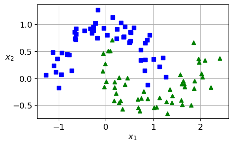
from sklearn.datasets import make_moons

X, y = make_moons(n_samples=100, noise=0.15, random_state=42)

plt.rcParams.update({'font.size': 12, "figure.figsize": (5,3)})

plt.plot(X[:, 0][y==0], X[:, 1][y==0], "bs")
plt.plot(X[:, 0][y==1], X[:, 1][y==1], "g^")
plt.grid(True)
plt.xlabel("$x_1$")
plt.ylabel("$x_2$", rotation=0)
plt.show()
from sklearn.pipeline import make_pipeline
from sklearn.preprocessing import StandardScaler
from sklearn.svm import SVC
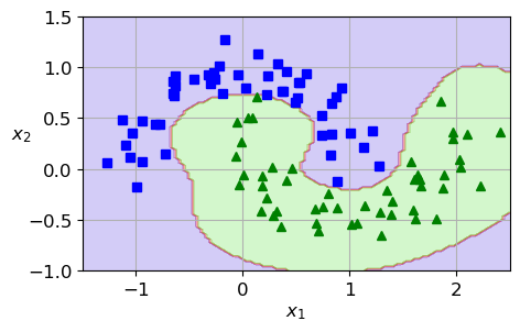
rbf_kernel_svm_clf = make_pipeline(StandardScaler(),
SVC(kernel="rbf", gamma=1, C=1e5)) # try 1e-5
rbf_kernel_svm_clf.fit(X, y)
Pipeline(steps=[('standardscaler', StandardScaler()),
                ('svc', SVC(C=100000.0, gamma=1))])
In a Jupyter environment, please rerun this cell to show the HTML representation or trust the notebook. On GitHub, the HTML representation is unable to render, please try loading this page with nbviewer.org.
Pipeline(steps=[('standardscaler', StandardScaler()),
('svc', SVC(C=100000.0, gamma=1))])StandardScaler()
SVC(C=100000.0, gamma=1)
def plot_dataset(X, y, axes):
    plt.plot(X[:, 0][y==0], X[:, 1][y==0], "bs")
    plt.plot(X[:, 0][y==1], X[:, 1][y==1], "g^")
    plt.axis(axes)
    plt.grid(True)
    plt.xlabel("$x_1$")
    plt.ylabel("$x_2$", rotation=0)
def plot_predictions(clf, axes):
    x0s = np.linspace(axes[0], axes[1], 100)
    x1s = np.linspace(axes[2], axes[3], 100)
    x0, x1 = np.meshgrid(x0s, x1s)
    X = np.c_[x0.ravel(), x1.ravel()]
    y_pred = clf.predict(X).reshape(x0.shape)
    plt.contourf(x0, x1, y_pred, cmap=plt.cm.brg, alpha=0.2)
plot_predictions(rbf_kernel_svm_clf, [-1.5, 2.5, -1, 1.5])
plot_dataset(X, y, [-1.5, 2.5, -1, 1.5])
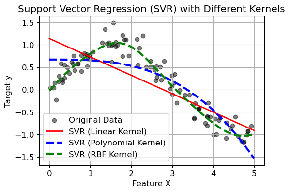
3. SVMs for regression#
Instead of trying to fit the largest possible street between two classes while limiting margin violations, SVM regression tries to fit as many instances as possible on the street while limiting margin violations
You can use the SVR class, which is the regression equivalent of the SVC class
Documentation: https://scikit-learn.org/stable/modules/generated/sklearn.svm.SVR.html
Epsilon in the epsilon-SVR model. It specifies the epsilon-tube within which no penalty is associated in the training loss function with points predicted within a distance epsilon from the actual value.
import numpy as np
import matplotlib.pyplot as plt
from sklearn.svm import SVR
from sklearn.model_selection import train_test_split

# Step 1: Generate synthetic non-linear data
np.random.seed(42)  # For reproducibility
X = np.sort(5 * np.random.rand(100, 1), axis=0)  # Feature values (1D)
y = np.sin(X).ravel() + 0.2 * np.random.randn(100)  # Target values with noise

# Step 2: Split the dataset into training and testing sets
X_train, X_test, y_train, y_test = train_test_split(X, y, test_size=0.2, random_state=42)

# Step 3: Train SVR models with different kernels
svr_linear = SVR(kernel="linear", C=10, epsilon=.1)
svr_poly = SVR(kernel="poly", C=10, epsilon=.1, degree=3)
svr_rbf = SVR(kernel="rbf", C=10, epsilon=.1, gamma=0.5)

svr_linear.fit(X_train, y_train)
svr_poly.fit(X_train, y_train)
svr_rbf.fit(X_train, y_train)

# Step 4: Make predictions
X_plot = np.linspace(0, 5, 100).reshape(-1, 1)  # Generate smooth input for visualization
y_pred_linear = svr_linear.predict(X_plot)
y_pred_poly = svr_poly.predict(X_plot)
y_pred_rbf = svr_rbf.predict(X_plot)

# Step 5: Visualization
plt.figure(figsize=(6, 4))

# Plot original data points
plt.scatter(X, y, color="black", label="Original Data", alpha=0.5)

# Plot SVR predictions
plt.plot(X_plot, y_pred_linear, color="red", lw=2, label="SVR (Linear Kernel)")
plt.plot(X_plot, y_pred_poly, color="blue", lw=3, linestyle="dashed", label="SVR (Polynomial Kernel)")
plt.plot(X_plot, y_pred_rbf, color="green", lw=3, linestyle="dashed", label="SVR (RBF Kernel)")

# Customize plot
plt.xlabel("Feature X")
plt.ylabel("Target y")
plt.title("Support Vector Regression (SVR) with Different Kernels")
plt.legend()
plt.grid()
plt.show()