Unsupervised Learning#
Machine Learning Methods#
Module 5: Unsupervised Learning#
Instructor: Farhad Pourkamali#
Overview#
Unsupervised learning deals with \(\color{red}{\text{unlabeled data}}\), meaning the model is not provided with output labels during training
The goal is to identify patterns, structures, or relationships within the data without explicit guidance from labeled examples
Labeling data for supervised learning can be a time-consuming and expensive task, especially when dealing with large data sets or complex tasks that require domain expertise
Suppose we have a data set of MRI brain scans where each sample represents a patient, and our goal is to classify them into three categories:
Healthy
Early-stage Alzheimer’s
Late-stage Alzheimer’s
Since manually labeling MRI scans is costly, we can use unsupervised learning to group similar scans without human input. A recent paper in the Journal of Advances in Biomarker Sciences and Technology: https://www.sciencedirect.com/science/article/pii/S2543106424000152
Clustering methods aim to partition a data set into clusters or groups in such a way that data points within the same cluster are more similar to each other than to those in other clusters
There is no universal definition of what a cluster is
It depends on the context and different algorithms will capture different kinds of clusters
Thus, the notion of similarity is crucial in clustering methods
We cover three popular clustering techniques and evaluation strategies in this module
K-means clustering (https://youtu.be/0COGLR7hUvI)
(Video for the rest of this module: https://youtu.be/lJsVyPOk7Ug)
Density-Based Spatial Clustering of Applications with Noise (DBSCAN)
Gaussian mixtures
Evaluation
Internal measures (cohesion and separation): Silhouette Coefficient
External measures (compare with ground-truth labels): Normalized Mutual Information
1. K-means clustering#
Assume we have \(K\) cluster centers \(\boldsymbol{\mu}_k, k=1,\ldots,K,\) in \(\mathbb{R}^D\), so we can cluster the data by assigning each sample \(\mathbf{x}_n\) to its closest center
But, we don’t know the cluster centers, so we should minimize the following loss function
For a specific data point \(\mathbf{x}_n\), we can rewrite:
as a matrix-vector multiplication
The row vector of \(\mathbf{Z}\) corresponding to \(\mathbf{x}_n\) is:
Note that only one of these values is 1 (the rest are 0)
Each row of \(\mathbf{M}\) represents a cluster center \(\boldsymbol{\mu}_k\):
where each \(\boldsymbol{\mu}_k\) is a row vector in \(\mathbb{R}^D\)
Multiplying the row vector \([z_{n1}, z_{n2}, \dots, z_{nK}]\) with \(\mathbf{M}\) selects the assigned cluster:
Thus, our term simplifies as:
which is just:
where \(\mathbf{Z}_n\) is the row vector of \(\mathbf{Z}\) corresponding to \(\mathbf{x}_n\)
Hence, for the entire data set, we have:
\(\mathbf{X}\in\mathbb{R}^{N\times D}\) (data matrix), \(\mathbf{Z}\in[0,1]^{N\times K}\) (membership matrix), and \(\mathbf{M}\in\mathbb{R}^{K\times D}\) (matrix of cluster centers)
Frobenius norm: \(\|\mathbf{A}\|_F^2= \sum_{i}\sum_{j} a_{ij}^2\)
K-means clustering algorithm
Start by placing the centers randomly (pick \(K\) instances at random)
Iterate over the following two steps
Assign each instance to the cluster whose center is closest
Update each cluster center by computing the mean of instances in that cluster
import numpy as np
import matplotlib.pyplot as plt
from sklearn.datasets import make_blobs
from sklearn.cluster import KMeans
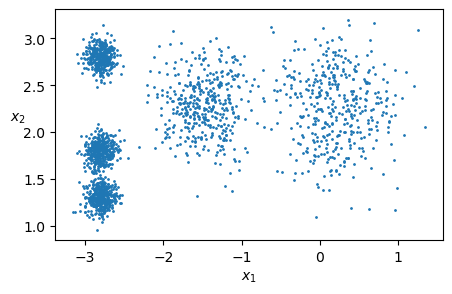
# We create a synthetic data set with 5 clusters or blobs
blob_centers = np.array([[ 0.2, 2.3], [-1.5 , 2.3], [-2.8, 1.8],
[-2.8, 2.8], [-2.8, 1.3]])
blob_std = np.array([0.4, 0.3, 0.1, 0.1, 0.1])
X, y = make_blobs(n_samples=2000, centers=blob_centers, cluster_std=blob_std,
random_state=7)
plt.rcParams.update({'font.size': 10, "figure.figsize": (5,3)})
plt.scatter(X[:, 0], X[:, 1], s=1)
plt.xlabel("$x_1$")
plt.ylabel("$x_2$", rotation=0)
plt.show()
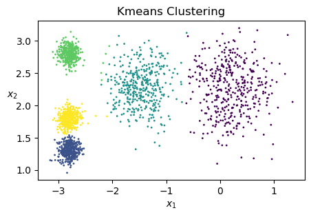
# Apply K-means clustering to this data set

# caveat: the number of clusters must be defined
kmeans = KMeans(n_clusters=5, random_state=1)

y_pred = kmeans.fit_predict(X)

plt.rcParams.update({'font.size': 10, "figure.figsize": (5,3)})
plt.scatter(X[:, 0], X[:, 1], c=y_pred, s=1)
plt.xlabel("$x_1$")
plt.ylabel("$x_2$", rotation=0)
plt.title('Kmeans Clustering')
plt.show()
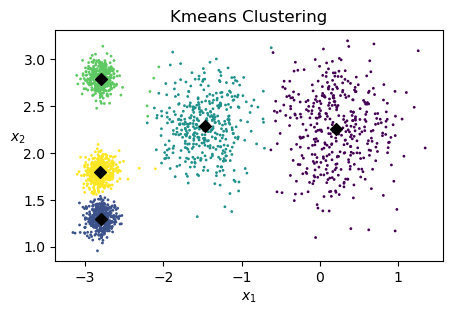
# find cluster centers
kmeans.cluster_centers_
array([[ 0.20876306,  2.25551336],
       [-2.80037642,  1.30082566],
       [-1.46679593,  2.28585348],
       [-2.79290307,  2.79641063],
       [-2.80389616,  1.80117999]])
# Plot cluster centers
plt.rcParams.update({'font.size': 10, "figure.figsize": (5,3)})
plt.scatter(X[:, 0], X[:, 1], c=y_pred, s=1)
plt.scatter(kmeans.cluster_centers_[:,0], kmeans.cluster_centers_[:,1], c='k', marker='D')
plt.xlabel("$x_1$")
plt.ylabel("$x_2$", rotation=0)
plt.title('Kmeans Clustering')
plt.show()
To create a K-Means model, specify the number of clusters and other optional parameters: https://scikit-learn.org/stable/modules/generated/sklearn.cluster.KMeans.html
# We can predict the labels of new instances

X_new = np.array([[0, 2], [3, 2], [-3, 3], [-3, 2.5]])
kmeans.predict(X_new)
array([0, 0, 3, 3], dtype=int32)
K-means clustering and initialization#
K-means clustering needs to be initialized carefully
Therefore, we can use multiple restarts, i.e., we run the algorithm multiple times from different random starting points, and then pick the best solution
Use the “n_init” argument
But, we can use better initialization techniques
The K-means++ algorithm
Pick the centers sequentially so as to “cover” the data
Each point is picked with probability proportional to its squared distance to its cluster center
Thus, at each iteration \(t\), we get
where
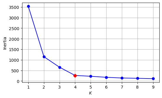
Finding the optimal number of clusters#
A natural choice for picking \(K\) is to pick the value that minimizes the reconstruction error
This is known as the inertia or within-cluster sum-of-squares criterion
This idea wouldn’t work because the inertia monotonically decreases with \(K\)
However, we can plot the inertia as a function of \(K\) and find the elbow
The elbow point is the value of \(K\) where adding more clusters no longer significantly reduces inertia
kmeans_per_k = [KMeans(n_clusters=k, random_state=42).fit(X)
                for k in range(1, 10)]
inertias = [model.inertia_ for model in kmeans_per_k]

plt.figure(figsize=(6, 3.5))
plt.plot(range(1, 10), inertias, "bo-")
plt.plot(4, inertias[3], 'rD')
plt.xlabel("$K$")
plt.ylabel("Inertia")
plt.grid()
plt.show()
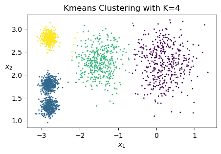
# solve the problem with K=4

kmeans = KMeans(n_clusters=4, random_state=1)

y_pred = kmeans.fit_predict(X)

plt.rcParams.update({'font.size': 10, "figure.figsize": (5,3)})
plt.scatter(X[:, 0], X[:, 1], c=y_pred, s=1)
plt.xlabel("$x_1$")
plt.ylabel("$x_2$", rotation=0)
plt.title('Kmeans Clustering with K=4')
plt.show()
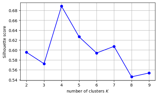
Using silhouette score instead of inertia#
The Silhouette Score evaluates clustering quality by measuring how well-separated clusters are. For each data point \(\mathbf{x}_n\), we compute:
\(a_n\) (Intra-cluster distance): The average distance from \(\mathbf{x}_n\) to all other points in the same cluster.
\(b_n\) (Inter-cluster distance): The average distance from \(\mathbf{x}_n\) to the nearest neighboring cluster (the closest cluster it is not part of).
The Silhouette Coefficient for each data point is defined as:
where:
\(-1 \leq s_n \leq 1\),
\(s_n \approx 1\) indicates well-clustered points (well-separated clusters),
\(s_n \approx 0\) suggests overlapping clusters,
\(s_n \approx -1\) indicates misclassified points.
Finally, the overall Silhouette Score is the average across all data points:
where \(N\) is the total number of samples
from sklearn.metrics import silhouette_score

silhouette_scores = [silhouette_score(X, model.labels_)
                     for model in kmeans_per_k[1:]]

plt.figure(figsize=(6, 3.5))
plt.plot(range(2, 10), silhouette_scores, "bo-")
plt.xlabel("number of clusters $K$")
plt.ylabel("Silhouette score")
plt.grid()
plt.show()
2. DBSCAN#
This algorithm defines clusters as continuous regions of high density
For each instance, it counts how many samples are located within a small distance \(\varepsilon\) from it (\(\varepsilon\)-neighborhood)
If an instance has at least “min_samples” samples in its \(\varepsilon\)-neighborhood, then it is considered a “core instance”
All instances in the neighborhood of a core instance belong to the same cluster
Any instance that is not a “core instance” and does not have one in its neighborhood is considered an anomaly
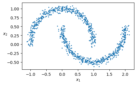
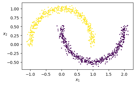
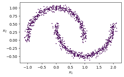
# Create a nonlinear data set

from sklearn.datasets import make_moons

X, y = make_moons(n_samples=1000, noise=0.05, random_state=42)

plt.rcParams.update({'font.size': 10, "figure.figsize": (5,3)})
plt.scatter(X[:, 0], X[:, 1], s=2)
plt.xlabel("$x_1$")
plt.ylabel("$x_2$", rotation=0)
plt.show()
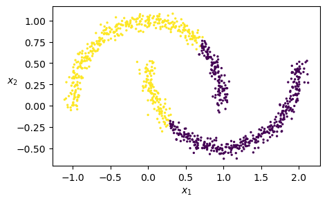
# Does K-means clustering work?

km = KMeans(n_clusters=2,  random_state=42)
km.fit(X)

plt.scatter(X[:, 0], X[:, 1], c=km.labels_, s=2)
plt.xlabel("$x_1$")
plt.ylabel("$x_2$", rotation=0)
plt.show()
from sklearn.cluster import DBSCAN

dbscan = DBSCAN(eps=0.2, min_samples=5)

dbscan.fit(X)

plt.scatter(X[:, 0], X[:, 1], c=dbscan.labels_, s=2)
plt.xlabel("$x_1$")
plt.ylabel("$x_2$", rotation=0)
plt.show()
# Does DBSCAN work with this value of eps?

dbscan = DBSCAN(eps=0.5, min_samples=5)
dbscan.fit(X)

plt.scatter(X[:, 0], X[:, 1], c=dbscan.labels_, s=2)
plt.xlabel("$x_1$")
plt.ylabel("$x_2$", rotation=0)
plt.show()
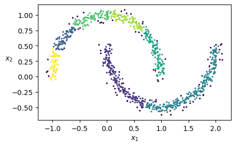
# Does DBSCAN work with this value of eps?

dbscan = DBSCAN(eps=0.05, min_samples=5)
dbscan.fit(X)

plt.scatter(X[:, 0], X[:, 1], c=dbscan.labels_, s=2)
plt.xlabel("$x_1$")
plt.ylabel("$x_2$", rotation=0)
plt.show()
3. Gaussian Mixtures#
The Gaussian Mixture Model (GMM) assumes that the data is generated from a mixture of multiple Gaussian distributions, each representing a cluster
The goal of the GMM is to identify these Gaussian distributions and estimate their parameters to assign data points to the most probable clusters
\(\pi_k\) is the mixing coefficient of the \(k\)-th Gaussian component, representing the probability of selecting the \(k\)-th component - If \(\pi_k\) is high, cluster \(k\) is dominant in the data set - If \(\pi_k\) is low, cluster \(k\) is rare
\(\boldsymbol{\mu}_k\) is the mean vector of the \(k\)-th Gaussian component
\(\boldsymbol{\Sigma}_k\) is the covariance matrix of the \(k\)-th Gaussian component
\(\mathcal{N}(\mathbf{x} | \boldsymbol{\mu}_k, \boldsymbol{\Sigma}_k)\) is the probability density function of the multivariate Gaussian distribution with mean \(\boldsymbol{\mu}_k\) and covariance \(\boldsymbol{\Sigma}_k\)
Unlike K-Means, where a data point is assigned to exactly one cluster, GMM assigns a probability of belonging to each cluster
The probability that \(\mathbf{x}\) belongs to the \(k\)-th cluster is given by:
Each data point has a soft assignment (probability) to multiple clusters, rather than a hard assignment.
Thus, GMM allows for overlapping clusters, making it more flexible than K-Means.
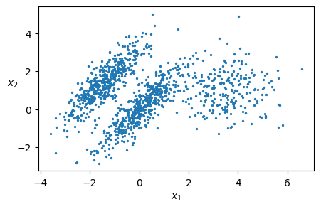
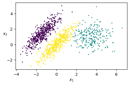
# create a 2D data set in the form of a mixture model
# Thus, we use make_blobs two times

X1, y1 = make_blobs(n_samples=1000, centers=((4, -4), (0, 0)), random_state=42)

X1 = X1.dot(np.array([[0.374, 0.95], [0.732, 0.598]]))

X2, y2 = make_blobs(n_samples=250, centers=1, random_state=42)

X2 = X2 + [6, -8]

X = np.r_[X1, X2]
y = np.r_[y1, y2]

plt.rcParams.update({'font.size': 10, "figure.figsize": (5,3)})
plt.scatter(X[:, 0], X[:, 1], s=2)
plt.xlabel("$x_1$")
plt.ylabel("$x_2$", rotation=0)
plt.show()
from sklearn.mixture import GaussianMixture

# number of clusters should be provided
gm = GaussianMixture(n_components=3, n_init=10, random_state=42)

gm.fit(X)
GaussianMixture(n_components=3, n_init=10, random_state=42)In a Jupyter environment, please rerun this cell to show the HTML representation or trust the notebook.
On GitHub, the HTML representation is unable to render, please try loading this page with nbviewer.org.
GaussianMixture(n_components=3, n_init=10, random_state=42)
# pi_k

gm.weights_
array([0.40005972, 0.20961444, 0.39032584])
# sigma_k

gm.covariances_
array([[[ 0.63478217,  0.72970097],
        [ 0.72970097,  1.16094925]],

       [[ 1.14740131, -0.03271106],
        [-0.03271106,  0.95498333]],

       [[ 0.68825143,  0.79617956],
        [ 0.79617956,  1.21242183]]])
# Plot returned clusters
y_pred = gm.fit_predict(X)

plt.scatter(X[:, 0], X[:, 1], c=y_pred, s=2)
plt.xlabel("$x_1$")
plt.ylabel("$x_2$", rotation=0)
plt.show()
gm.fit_predict(X)[:10]
array([2, 2, 0, 2, 0, 0, 2, 0, 0, 2])
gm.predict_proba(X)[:10]
array([[6.76282339e-07, 2.31833274e-02, 9.76815996e-01],
       [6.74575575e-04, 1.64110061e-02, 9.82914418e-01],
       [9.99922764e-01, 1.99781831e-06, 7.52377580e-05],
       [8.64003688e-06, 8.48983970e-03, 9.91501520e-01],
       [9.99999975e-01, 2.31088296e-08, 2.35665725e-09],
       [9.93716619e-01, 3.52304610e-04, 5.93107648e-03],
       [2.47914411e-11, 6.56144058e-03, 9.93438559e-01],
       [9.68375227e-01, 5.77260043e-04, 3.10475133e-02],
       [9.99990891e-01, 8.70189912e-06, 4.07452914e-07],
       [7.37064964e-05, 1.51236024e-03, 9.98413933e-01]])
4. Evaluating Clustering with Normalized Mutual Information (NMI)#
In classification, we have ground truth labels and predicted labels, so accuracy is a natural evaluation metric:
However, in clustering, we do not have predefined class labels. Instead:
Clustering assigns data points to clusters without knowing their true class labels.
Cluster labels are arbitrary (e.g., swapping “Cluster A” and “Cluster B” does not change the clustering).
Accuracy depends on exact label matching, which is not meaningful for clustering.
Thus, we need a label-independent metric to measure how well clusters match ground truth groups.
Solution: Normalized Mutual Information (NMI)
NMI measures the mutual dependence between true labels and cluster assignments.
It is invariant to label permutations.
NMI provides a normalized score between 0 and 1, where:
NMI = 1 means perfect clustering.
NMI = 0 means no correlation between clusters and true labels.
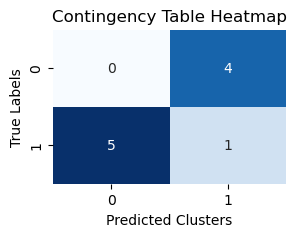
Contingency Table#
A contingency table (also called a confusion matrix for clustering) represents the relationship between true labels and predicted clusters.
Each entry \(C(i, j)\) in the table represents the number of data points that belong to true class \(i\) but were assigned to predicted cluster \(j\).

Rows represent true labels (ground truth).
Columns represent predicted clusters.
The values in the table indicate how many points from each true label were assigned to each cluster.
This table allows us to compute:
Entropy of True Label \(H(Y)\)
Entropy of Predicted Clusters \(H(\hat{Y})\)
Mutual Information (MI) between true and predicted labels.
Normalized Mutual Information (NMI) by normalizing MI.
Step 1: Compute Entropy of True Labels#
Entropy measures the uncertainty or randomness in the distribution of true labels. It is given by:
where:
\(P(y)\) is the probability of each true label.
Higher entropy means more diverse true labels.
From the contingency table, we compute:
where:
\(|Y_i|\) is the number of samples in each true class,
\(N\) is the total number of data points.
Step 2: Compute Entropy of Predicted Labels#
Similarly, the entropy of predicted clusters is:
where:
\(P(\hat{y})\) is the probability of each predicted cluster.
We compute it using the column sums of the contingency table.
Step 3: Compute Mutual Information#
Mutual Information (MI) quantifies how much knowing the predicted cluster reduces uncertainty about the true label:
where:
\(P(y, \hat{y})\) is the joint probability (computed from the contingency table).
If \(P(y, \hat{y})\) is high, clustering aligns well with ground truth.
Step 4: Compute Normalized Mutual Information (NMI)#
To ensure values range from 0 to 1, we normalize MI:
import numpy as np
import pandas as pd
import matplotlib.pyplot as plt
import seaborn as sns
from sklearn.metrics import normalized_mutual_info_score

# Define true labels and predicted cluster assignments
true_labels = np.array([0, 1, 1, 1, 1, 0, 1, 0, 1, 0])
predicted_clusters = np.array([1, 1, 0, 0, 0, 1, 0, 1, 0, 1])  # Different label ordering

print('\n',true_labels, '\n', predicted_clusters)

# Step 1: Compute the contingency table (confusion matrix for clustering)
contingency_table = pd.crosstab(pd.Series(true_labels, name='True Labels'),
                                pd.Series(predicted_clusters, name='Predicted Clusters'))


# Visualizing the contingency table as a heatmap
plt.figure(figsize=(3, 2))
sns.heatmap(contingency_table, annot=True, fmt="d", cmap="Blues", cbar=False)
plt.xlabel("Predicted Clusters")
plt.ylabel("True Labels")
plt.title("Contingency Table Heatmap")
plt.show()
 [0 1 1 1 1 0 1 0 1 0]
 [1 1 0 0 0 1 0 1 0 1]
# Step 2: Compute entropy of true labels H(Y)
p_y = contingency_table.sum(axis=1) / contingency_table.values.sum()
H_Y = -np.sum(p_y * np.log2(p_y))

print(p_y, H_Y)
True Labels
0    0.4
1    0.6
dtype: float64 0.9709505944546686
# Step 3: Compute entropy of predicted labels H(Y_hat)
p_y_hat = contingency_table.sum(axis=0) / contingency_table.values.sum()
H_Y_hat = -np.sum(p_y_hat * np.log2(p_y_hat))

print(p_y_hat, H_Y_hat)
Predicted Clusters
0    0.5
1    0.5
dtype: float64 1.0
# Step 4: Compute mutual information MI(Y, Y_hat)
joint_prob = contingency_table / contingency_table.values.sum()
p_joint = joint_prob.values

# Avoid log(0) issue by setting zeros to a small value before applying log
p_joint = np.where(p_joint == 0, 1e-10, p_joint)
p_y = np.where(p_y == 0, 1e-10, p_y)
p_y_hat = np.where(p_y_hat == 0, 1e-10, p_y_hat)

MI = np.sum(p_joint * np.log2(p_joint / (p_y[:, None] * p_y_hat[None, :])))

print(MI)
0.6099865439212522
# Step 5: Compute normalized mutual information (NMI)
NMI = MI / np.sqrt(H_Y * H_Y_hat)

# Compute NMI using sklearn for comparison
NMI_sklearn = normalized_mutual_info_score(true_labels, predicted_clusters)

print(f"Normalized Mutual Information (NMI - Manual): {NMI:.4f}")
print(f"Normalized Mutual Information (NMI - sklearn): {NMI_sklearn:.4f}")
Normalized Mutual Information (NMI - Manual): 0.6190
Normalized Mutual Information (NMI - sklearn): 0.6190
from sklearn import datasets
from sklearn.cluster import KMeans
from sklearn.metrics import normalized_mutual_info_score
import matplotlib.pyplot as plt

# Load the Iris dataset
iris = datasets.load_iris()
X = iris.data  # Features (sepal length, sepal width, petal length, petal width)
y_true = iris.target  # True labels (0: Setosa, 1: Versicolor, 2: Virginica)

# Apply K-Means clustering (without using true labels)
kmeans = KMeans(n_clusters=3, random_state=42, n_init=10)
y_pred = kmeans.fit_predict(X)  # Cluster assignments

# Compute NMI Score
nmi_score = normalized_mutual_info_score(y_true, y_pred)

# Visualizing clustering results (Sepal Length vs Sepal Width)
plt.figure(figsize=(5, 4))
plt.scatter(X[:, 0], X[:, 1], c=y_pred, cmap='viridis', alpha=0.6, label="Clusters")
plt.scatter(kmeans.cluster_centers_[:, 0], kmeans.cluster_centers_[:, 1], c='red', marker='X', s=100, label="Centroids")
plt.xlabel("Sepal Length")
plt.ylabel("Sepal Width")
plt.title("K-Means Clustering on Iris Dataset")
plt.legend()
plt.show()

# Print the computed NMI Score
print(f"Normalized Mutual Information (NMI): {nmi_score:.4f}")
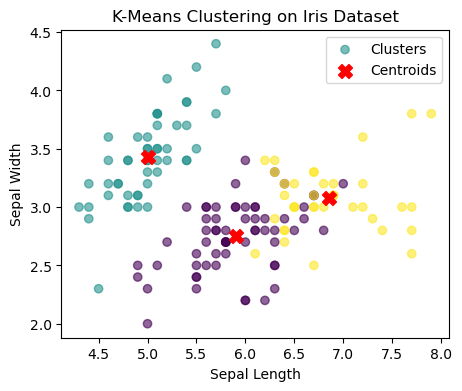
Normalized Mutual Information (NMI): 0.7582