Gradient Boosting

Gradient Boosting#

Machine Learning Methods#

Module 6: Advanced Machine Learning Models#

Part 3: Random Forest vs. Gradient Boosting#

Instructor: Farhad Pourkamali#

Overview#

Video: https://youtu.be/xZw-hWRpt2A
Ensemble learning combines multiple base models to improve overall performance and robustness.
Two popular ensemble techniques are Bagging (Bootstrap Aggregating) and Boosting.
- Bagging builds multiple independent models in parallel using bootstrapped (resampled) datasets and averages their predictions to reduce variance.
- Boosting builds models sequentially, where each new model focuses on correcting the errors of the previous ones, reducing bias and improving accuracy.
These techniques are especially effective when combining weak learners—models that perform slightly better than random chance.

In this notebook, we focus on using Decision Trees as base models for Bagging and Boosting. However, these techniques are versatile and can be applied to other machine learning models as well.

import numpy as np
import matplotlib.pyplot as plt
from sklearn.tree import DecisionTreeRegressor, plot_tree

# 1. Generate synthetic data: noisy sine wave
np.random.seed(42)
X = np.sort(np.random.rand(80, 1) * 5, axis=0)
y = np.sin(X).ravel() + np.random.normal(0, 0.1, size=X.shape[0])

# 2. Generate test data for smooth plotting
X_test = np.linspace(0, 5, 500).reshape(-1, 1)

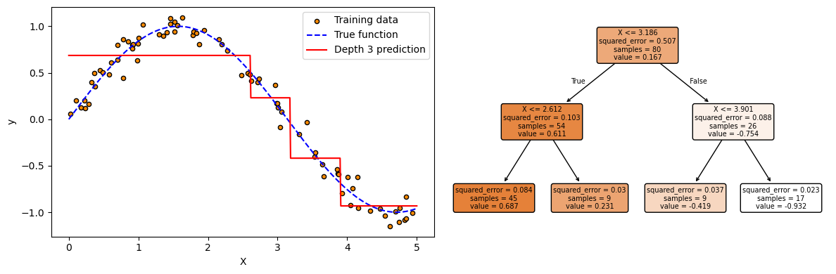
# 3. Fit model with max_depth=2
model = DecisionTreeRegressor(max_depth=2, random_state=0)
model.fit(X, y)
y_pred = model.predict(X_test)

# 4. Plot vertically: Prediction on top, tree below
plt.figure(figsize=(12, 4))

# Prediction plot
plt.subplot(1, 2, 1)
plt.scatter(X, y, s=20, edgecolor="k", c="darkorange", label="Training data")
plt.plot(X_test, np.sin(X_test), "b--", label="True function")
plt.plot(X_test, y_pred, "r", label="Depth 3 prediction")
plt.xlabel("X")
plt.ylabel("y")
plt.legend()

# Tree structure
plt.subplot(1, 2, 2)
plot_tree(model, filled=True, rounded=True, feature_names=["X"], fontsize=7)

plt.tight_layout()
plt.show()

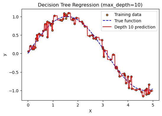
../_images/810a01cf73bf729b152d4673ef60dbe531bda4ffaad96820d12543fb6f9cfd88.png

# 3. Fit model with max_depth=10
model = DecisionTreeRegressor(max_depth=10, random_state=0)
model.fit(X, y)
y_pred = model.predict(X_test)

# 4. Plot vertically: Prediction on top, tree below
plt.figure(figsize=(6, 4))

# Prediction plot
plt.scatter(X, y, s=20, edgecolor="k", c="darkorange", label="Training data")
plt.plot(X_test, np.sin(X_test), "b--", label="True function")
plt.plot(X_test, y_pred, "r", label="Depth 10 prediction")
plt.title("Decision Tree Regression (max_depth=10)")
plt.xlabel("X")
plt.ylabel("y")
plt.legend()
plt.show()

../_images/4a5a6810fd272064d33947451ee1c27b78096190f677b0b78081993ec9b0a5ae.png

1. Bagging (Bootstrap Aggregating) Algorithm#

Bagging is an ensemble method that builds multiple models on different bootstrapped subsets of the data and combines their outputs, typically by averaging (for regression) or majority vote (for classification).

Algorithm: Bagging (for Regression)

Input: Training dataset $\mathcal{D}$ with $n$ samples, number of models $B$ (typically $B = 100$)
For $b = 1, \ldots, B$:
- Sample a bootstrap dataset $\mathcal{D}_b$ from $\mathcal{D}$ (i.e., sample $n$ points with replacement)
- Train a base model $f^{(b)}(x)$ on $\mathcal{D}_b$
Output: The final bagged prediction is: $$ f^{\text{bagging}}(x) = \frac{1}{B} \sum_{b=1}^B f^{(b)}(x) $$

Random Forest: Bagging + Feature Randomness#

Random Forests build on the idea of bagging by also introducing randomness at the feature level to reduce correlation between individual trees:

At each split in a decision tree, instead of considering all $p$ features, a random subset of features is selected.
For classification tasks, this subset size is usually $\sqrt{p}$.
This extra layer of randomness ensures that the individual trees are decorrelated, making the ensemble more effective.

import numpy as np
import matplotlib.pyplot as plt
from sklearn.tree import DecisionTreeRegressor
from sklearn.ensemble import RandomForestRegressor

# 1. Generate synthetic data: noisy sine wave
np.random.seed(42)
X = np.sort(np.random.rand(80, 1) * 5, axis=0)
y = np.sin(X).ravel() + np.random.normal(0, 0.1, size=X.shape[0])

# 2. Generate test data for smooth plotting
X_test = np.linspace(0, 5, 500).reshape(-1, 1)

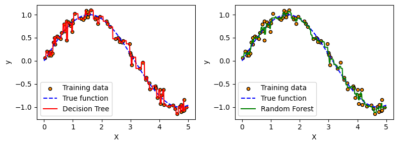
# 3. Fit a single Decision Tree (depth 10)
dt_model = DecisionTreeRegressor(max_depth=10, random_state=0)
dt_model.fit(X, y)
dt_pred = dt_model.predict(X_test)

# 4. Fit a Random Forest with 100 trees (depth 10)
rf_model = RandomForestRegressor(n_estimators=100, max_depth=10, random_state=0)
rf_model.fit(X, y)
rf_pred = rf_model.predict(X_test)

# 5. Plot predictions
plt.figure(figsize=(8, 3))

# Top: Decision Tree
plt.subplot(1, 2, 1)
plt.scatter(X, y, s=20, edgecolor="k", c="darkorange", label="Training data")
plt.plot(X_test, np.sin(X_test), "b--", label="True function")
plt.plot(X_test, dt_pred, "r", label="Decision Tree")
plt.xlabel("X")
plt.ylabel("y")
plt.legend()

# Bottom: Random Forest
plt.subplot(1, 2, 2)
plt.scatter(X, y, s=20, edgecolor="k", c="darkorange", label="Training data")
plt.plot(X_test, np.sin(X_test), "b--", label="True function")
plt.plot(X_test, rf_pred, "g", label="Random Forest")
plt.xlabel("X")
plt.ylabel("y")
plt.legend()

plt.tight_layout()
plt.show()

../_images/2e35e3af07ab0afaf184dead5b6dc5abb6a34065044995db9726f840ba604530.png

2. Mean Decrease Impurity (MDI)#

Random Forests build numerous decision trees, making direct visualization and interpretation challenging.
MDI provides a way to distill the complex model into a simple, interpretable feature importance metric.
Impurity Reduction
- Each tree evaluates features to minimize “impurity” at each node split.
- The definition of impurity depends on the task:
```
- Classification: Gini Index or Entropy
- Regression: Variance (often via Mean Squared Error)
```
- When a feature is used to split a node, it reduces the impurity — this reduction is recorded as its contribution.
MDI averages the impurity reduction attributed to each feature across all trees in the forest.
This results in a robust, aggregated estimate of how important each feature is to the model’s predictions.
Features with higher MDI values are considered more important.

import numpy as np
import matplotlib.pyplot as plt
from sklearn.datasets import load_diabetes
from sklearn.ensemble import RandomForestRegressor
from sklearn.model_selection import train_test_split
from sklearn.metrics import r2_score

# Load dataset
diabetes = load_diabetes()
X = diabetes.data
y = diabetes.target
feature_names = diabetes.feature_names

# Train/test split
X_train, X_test, y_train, y_test = train_test_split(X, y, random_state=42)

# Train Random Forest Regressor
rf = RandomForestRegressor(n_estimators=100, max_depth=10, random_state=42)
rf.fit(X_train, y_train)

# Evaluate
y_pred = rf.predict(X_test)
r2 = r2_score(y_test, y_pred)
print(f"R2 score: {r2:.2f}")

# Feature importances
importances = rf.feature_importances_
indices = np.argsort(importances)[::-1]

# Plot feature importances
plt.figure(figsize=(7, 4))
plt.bar(range(X.shape[1]), importances[indices], align="center")
plt.xticks(range(X.shape[1]), [feature_names[i] for i in indices], rotation=45)
plt.ylabel("Importance Score")
plt.tight_layout()
plt.show()

R2 score: 0.46

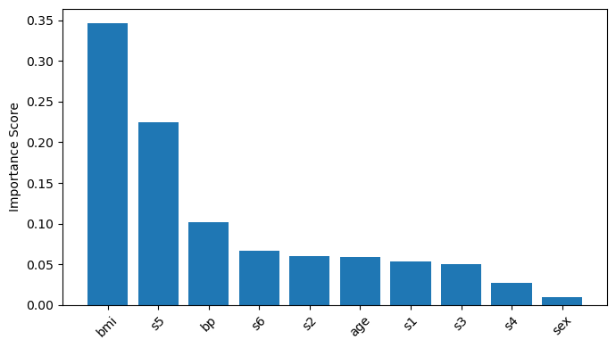
../_images/9e7f27d16db015090c22f44fd6134689f9a08a02937b4d1eff40059ad7c57542.png

List of features for this dataset:
- age: Age in years
- sex
- bmi: Body Mass Index
- bp: Average blood pressure
- s1: TC, total serum cholesterol
- s2: LDL, low-density lipoproteins
- s3: HDL, high-density lipoproteins
- s4: TCH, total cholesterol / HDL
- s5: LTG, possibly log of serum triglycerides level
- s6: GLU, blood sugar level

3. Boosting#

Like bagging, boosting is a general ensemble approach that can be applied to many machine learning methods.
Unlike bagging, boosting trains models sequentially, not in parallel.
Boosting does not involve bootstrapping (sampling with replacement); instead, each tree is trained on a modified version of the original dataset.
At each step, a new model is trained to fit the residuals (errors) of the current model.
This means the new decision tree is fit not to the original outputs, but to the errors made by the current ensemble.
The new tree is then added to the existing model, and the residuals are updated.

Algorithm: Boosting (for Regression)

Initialize the model:
- Set the initial prediction:
  $$ \hat{f}(x) = 0 $$
- Set residuals for all training points:
  $$ r_i = y_i \quad \text{for all } i $$
For $b = 1, 2, \ldots, B$, repeat:

a. Fit a regression tree $\hat{f}^b$ with $d$ splits to the residuals $r$ using the training data $(X, r)$.

b. Update the model by adding a scaled version of the new tree:
$$ \hat{f}(x) \leftarrow \hat{f}(x) + \lambda \hat{f}^b(x) $$

c. Update the residuals:
$$ r_i \leftarrow r_i - \lambda \hat{f}^b(x_i) $$
Output the final boosted model:
$$ \hat{f}(x) = \sum_{b=1}^{B} \lambda \hat{f}^b(x) $$

$\lambda$ is the learning rate (typically small, like 0.01), which controls how much each tree contributes.

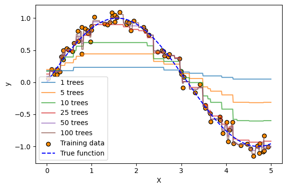
Gradient Boosting – Extension of Boosting#

Gradient Boosting generalizes the boosting algorithm by allowing optimization of any differentiable loss function.
Instead of using raw residuals, it fits each new model to the negative gradient of the loss function, called pseudo-residuals.

Pseudo-Residuals: For each data point $x_i$, the pseudo-residual at boosting step $b$ is:

\[ r_{ib} = -\left[ \frac{\partial L(y_i, \hat{f}(x_i))}{\partial \hat{f}(x_i)} \right]_{\hat{f}(x) = \hat{f}_{b-1}(x)} \]

Where:
- $L(y_i, \hat{f}(x_i))$ is the loss function (e.g., squared error, huber loss).
- $\hat{f}_{b-1}(x_i)$ is the model prediction from the previous iteration.
- $r_{ib}$ is the negative gradient — the direction in which the model should adjust its prediction to reduce the loss.

For the squared error (quadratic loss), the loss function for a single data point is:

\[ L(y_i, \hat{f}(x_i)) = \frac{1}{2} (y_i - \hat{f}(x_i))^2 \]

\[ r_{ib} = -\frac{\partial L(y_i, \hat{f}(x_i))}{\partial \hat{f}(x_i)}= -(- (y_i - \hat{f}(x_i))) = y_i - \hat{f}(x_i) \]

import numpy as np
import matplotlib.pyplot as plt
from sklearn.ensemble import GradientBoostingRegressor

# 1. Generate synthetic data: noisy sine wave
np.random.seed(42)
X = np.sort(np.random.rand(80, 1) * 5, axis=0)
y = np.sin(X).ravel() + np.random.normal(0, 0.1, size=X.shape[0])

# 2. Generate test data for smooth plotting
X_test = np.linspace(0, 5, 500).reshape(-1, 1)

# 3. Fit Gradient Boosting Regressor
gbr = GradientBoostingRegressor(n_estimators=100, learning_rate=0.1, max_depth=3, random_state=42)
gbr.fit(X, y)

# 4. Plot the growth of predictions over iterations
plt.figure(figsize=(6, 4))
for i, y_pred in enumerate(gbr.staged_predict(X_test)):
    if i in [0, 4, 9, 24, 49, 99]:  # select a few iterations to plot
        plt.plot(X_test, y_pred, label=f"{i+1} trees", alpha=0.7)

# Plot original data and true function
plt.scatter(X, y, c="darkorange", edgecolor="k", label="Training data")
plt.plot(X_test, np.sin(X_test), "b--", label="True function")
plt.xlabel("X")
plt.ylabel("y")
plt.legend()
plt.tight_layout()
plt.show()

../_images/be96b20c123be23b487aaa88a0f6c747c0505ed0e495553c54adc4c2edab58e4.png