Parametric Regression Models#
Machine Learning Methods#
Module 3: Parametric Regression Models#
Instructor: Farhad Pourkamali#
Overview#
Linear regression: Problem formulation, assumption, loss function, gradient (https://youtu.be/7bzSIX2I2Uk)
Linear regression in Scikit-learn (https://youtu.be/faW0Zo9CTQ8)
Evaluation metrics (https://youtu.be/faW0Zo9CTQ8)
Gradient descent (GD) and variants (https://youtu.be/0EV6UoKM4AM)
Nonlinear extension and regularization (https://youtu.be/OIoe4OQo1ko)

1. Linear regression: Problem formulation, assumption, loss function, gradient#
Case study: univariate linear regression#
Training data: \(\mathcal{D}=\{(x_n,y_n)\}_{n=1}^N\)
Parametric model: \(f(x)=\theta_0+\theta_1 x\)
Objective: Choose \(\theta_0,\theta_1\) such that \(f(x_n)\) is close to \(y_n\)
Mean squared error (MSE):
Solving the optimization problem#
We’ll need the concept of partial derivatives
To compute \(\partial \mathcal{L}/\partial \theta_0\), take the derivative with respect to \(\theta_0\), treating the rest of the arguments as constants
We can show that
Gradient#
Extend the notion of derivatives to handle vector-argument functions
Given \(\mathcal{L}:\mathbb{R}^d\mapsto \mathbb{R}\), where \(d\) is the number of input variables
\[\begin{split}\nabla \mathcal{L}=\begin{bmatrix}\frac{\partial \mathcal{L}}{\partial \theta_0}\\ \vdots\\ \frac{\partial \mathcal{L}}{\partial \theta_{d-1}} \end{bmatrix}\in\mathbb{R}^d\end{split}\]Example from the previous slide (\(d=2\)):
Compact form of gradient#
Let us define
Hence, we get
Compact form of gradient#
The last step is to show that \(\nabla \mathcal{L}\) can be written as
Given this compact form, we can use NumPy to solve the linear matrix equation
# GDP data
import numpy as np
import pandas as pd
import matplotlib.pyplot as plt

df = pd.read_csv("https://github.com/ageron/data/raw/main/lifesat/lifesat.csv")

df.head()
| Country | GDP per capita (USD) | Life satisfaction | |
|---|---|---|---|
| 0 | Russia | 26456.387938 | 5.8 |
| 1 | Greece | 27287.083401 | 5.4 |
| 2 | Turkey | 28384.987785 | 5.5 |
| 3 | Latvia | 29932.493910 | 5.9 |
| 4 | Hungary | 31007.768407 | 5.6 |
df.info()
<class 'pandas.core.frame.DataFrame'>
RangeIndex: 27 entries, 0 to 26
Data columns (total 3 columns):
 #   Column                Non-Null Count  Dtype
---  ------                --------------  -----
 0   Country               27 non-null     object
 1   GDP per capita (USD)  27 non-null     float64
 2   Life satisfaction     27 non-null     float64
dtypes: float64(2), object(1)
memory usage: 780.0+ bytes
# Input features and labels (or outcomes) for the regression problem

X = df['GDP per capita (USD)'].to_numpy()
y = df['Life satisfaction'].to_numpy()

print(X.shape, y.shape)
(27,) (27,)
X
array([26456.38793813, 27287.08340093, 28384.98778463, 29932.49391006,
       31007.76840654, 32181.15453723, 32238.15725928, 35638.42135118,
       36215.44759073, 36547.73895598, 36732.03474403, 38341.30757041,
       38992.14838075, 41627.12926943, 42025.61737306, 42404.39373816,
       45856.62562648, 47260.80045844, 48210.03311134, 48697.83702825,
       50683.32350972, 50922.35802345, 51935.60386182, 52279.72885136,
       54209.56383573, 55938.2128086 , 60235.7284917 ])
X.reshape(-1,1)
array([[26456.38793813],
       [27287.08340093],
       [28384.98778463],
       [29932.49391006],
       [31007.76840654],
       [32181.15453723],
       [32238.15725928],
       [35638.42135118],
       [36215.44759073],
       [36547.73895598],
       [36732.03474403],
       [38341.30757041],
       [38992.14838075],
       [41627.12926943],
       [42025.61737306],
       [42404.39373816],
       [45856.62562648],
       [47260.80045844],
       [48210.03311134],
       [48697.83702825],
       [50683.32350972],
       [50922.35802345],
       [51935.60386182],
       [52279.72885136],
       [54209.56383573],
       [55938.2128086 ],
       [60235.7284917 ]])
np.ones((X.shape[0],1))
array([[1.],
       [1.],
       [1.],
       [1.],
       [1.],
       [1.],
       [1.],
       [1.],
       [1.],
       [1.],
       [1.],
       [1.],
       [1.],
       [1.],
       [1.],
       [1.],
       [1.],
       [1.],
       [1.],
       [1.],
       [1.],
       [1.],
       [1.],
       [1.],
       [1.],
       [1.],
       [1.]])
# add the column of all 1's

def add_column(X):
    '''
    add the column of all 1's
    '''
    return np.concatenate(( np.ones((X.shape[0],1)), X.reshape(-1,1) ), axis=1)

Xcon = add_column(X)

Xcon.shape
(27, 2)
Xcon
array([[1.00000000e+00, 2.64563879e+04],
       [1.00000000e+00, 2.72870834e+04],
       [1.00000000e+00, 2.83849878e+04],
       [1.00000000e+00, 2.99324939e+04],
       [1.00000000e+00, 3.10077684e+04],
       [1.00000000e+00, 3.21811545e+04],
       [1.00000000e+00, 3.22381573e+04],
       [1.00000000e+00, 3.56384214e+04],
       [1.00000000e+00, 3.62154476e+04],
       [1.00000000e+00, 3.65477390e+04],
       [1.00000000e+00, 3.67320347e+04],
       [1.00000000e+00, 3.83413076e+04],
       [1.00000000e+00, 3.89921484e+04],
       [1.00000000e+00, 4.16271293e+04],
       [1.00000000e+00, 4.20256174e+04],
       [1.00000000e+00, 4.24043937e+04],
       [1.00000000e+00, 4.58566256e+04],
       [1.00000000e+00, 4.72608005e+04],
       [1.00000000e+00, 4.82100331e+04],
       [1.00000000e+00, 4.86978370e+04],
       [1.00000000e+00, 5.06833235e+04],
       [1.00000000e+00, 5.09223580e+04],
       [1.00000000e+00, 5.19356039e+04],
       [1.00000000e+00, 5.22797289e+04],
       [1.00000000e+00, 5.42095638e+04],
       [1.00000000e+00, 5.59382128e+04],
       [1.00000000e+00, 6.02357285e+04]])
np.concatenateExplanationPurpose:
Combines (concatenates) multiple arrays into a single array along a specified axis.
Input:
A tuple or list of arrays to concatenate, all with the same shape except in the concatenation axis.
Axis:
Defines the dimension along which the arrays will be joined.
Default: axis=0 (rows are stacked for 2D arrays).
For axis=1, arrays are concatenated column-wise.
Shape Requirement:
All arrays must have the same shape in dimensions other than the specified axis.
Output:
A new array that is the concatenation of the input arrays along the specified axis.
# solve the problem

a = np.matmul(np.transpose(Xcon), Xcon)

b = np.matmul(np.transpose(Xcon), y)

theta = np.linalg.lstsq(a, b, rcond=None)[0] # Cut-off ratio for small singular values

print(theta)
[3.74904943e+00 6.77889970e-05]
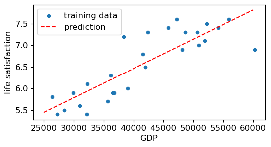
# plot the prediction model f

def f(X, theta):
    return np.matmul(X, theta)

plt.rcParams.update({'font.size': 12, "figure.figsize": (6,3)})
plt.scatter(X, y, s=20, label='training data')

X_test = np.array([25000, 60000])
y_test = f(add_column(X_test), theta)
plt.plot(X_test, y_test, 'r--', label='prediction')

plt.legend()
plt.xlabel('GDP')
plt.ylabel('life satisfaction')
plt.show()
Linear models for regression#
Given the training data set \(\mathcal{D}=\{(\mathbf{x}_n,y_n)\}_{n=1}^N\) and an input vector \(\mathbf{x}\in\mathbb{R}^D\), the linear regression model takes the form
\(\boldsymbol{\theta}\in\mathbb{R}^D\): weights or regression coefficients, \(\theta_0\): intercept or bias term
Compact representation by defining \(\mathbf{x}=[\color{red}{x_0=1},x_1,\ldots,x_D]\) and \(\boldsymbol{\theta}=[\theta_0,\theta_1,\ldots,\theta_D]\) in \(\mathbb{R}^{D+1}\)
Loss function for linear regression#
MSE loss function for a linear regression model
where we have
Optimization problem for model fitting/training: \(\underset{\boldsymbol{\theta}\in\mathbb{R}^{D+1}}{\operatorname{argmin}} \mathcal{L}(\boldsymbol{\theta})\)
The Normal equation#
To find the value of \(\boldsymbol{\theta}\) that minimizes the MSE, there exists a closed-form solution
a mathematical equation that gives the result directly
The gradient takes the form
Normal equation
2. Linear regression in Scikit-learn#
Import the
LinearRegressionclass fromsklearn.linear_model.Create an instance of the model.
from sklearn.linear_model import LinearRegression
model = LinearRegression()
Use the
.fit()method to train the model on your data.Pass the feature matrix (X) and target vector (y) to the method.
model.fit(X, y)
Use the
.predict()method to predict target values for new data points.
predictions = model.predict(new_X)
Attributes
.coef_: The coefficients (weights) for the linear equation..intercept_: The intercept term (bias) of the linear model.
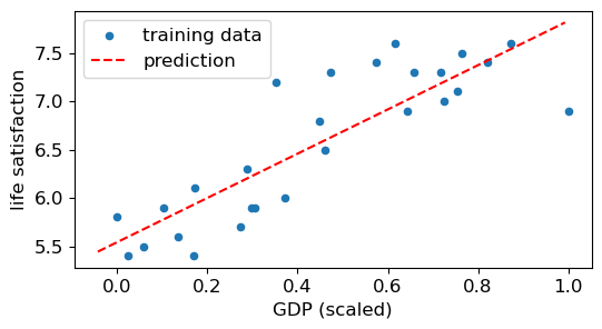
from sklearn.linear_model import LinearRegression

# Revisit the GDP data by preprocessing input features

from sklearn.preprocessing import MinMaxScaler

minmax = MinMaxScaler()

X_minmax = minmax.fit_transform(X.reshape(-1,1))

reg = LinearRegression()

reg.fit(X_minmax, y) # X should be a 2D array

print(reg.intercept_, reg.coef_)
5.542501428448674 [2.28986761]
# Plot the prediction model

plt.rcParams.update({'font.size': 12, "figure.figsize": (6,3)})
plt.scatter(X_minmax, y, s=20, label='training data')

X_test = np.array([25000, 60000]).reshape(-1,1)
X_test_minmax = minmax.transform(X_test)
plt.plot(X_test_minmax, reg.predict(X_test_minmax), 'r--', label='prediction')

plt.legend()
plt.xlabel('GDP (scaled)')
plt.ylabel('life satisfaction')
plt.show()
3. Evaluation metrics#
The quality of a regression model can be assessed using various quantities
Mean squared error
The value you get after calculating MSE is a squared unit of output
If you have outliers in the data set, then it penalizes the outliers most
Possible solution: the output value you get is in the same unit as the required output variable
from sklearn.metrics import mean_squared_error, root_mean_squared_error

y_true = [3, -1, 2, 7]
y_pred = [3, 0, 2, 7]

# If True returns MSE value, if False returns RMSE value.
print('MSE: ', mean_squared_error(y_true, y_pred),
      ', RMSE: ', root_mean_squared_error(y_true, y_pred))
MSE: 0.25 , RMSE: 0.5
R² score or the coefficient of determination#
Definition
RSS (Residual Sum of Squares) measures the amount of variability that is left unexplained
Best possible score is 1.
An \(R^2\) score of 0 in a regression model means that the model’s predictions are no better than simply predicting the mean of the target variable for all data points.
A negative \(R^2\) is a signal to revisit the model design or data preparation steps.
import numpy as np
from sklearn.linear_model import LinearRegression
from sklearn.metrics import r2_score

# Data where the model performs poorly
X = np.array([[1], [2], [3]])
y = np.array([10, 20, 30])  # Actual target values
y_bad_pred = np.array([40, 50, 60])  # Poor predictions

# Calculate R² manually
ss_res = np.sum((y - y_bad_pred)**2)  # Residual sum of squares
ss_tot = np.sum((y - np.mean(y))**2)  # Total sum of squares
r2 = 1 - (ss_res / ss_tot)

print("R² score:", r2)
R² score: -12.5
Explained variance score#
Definition
The best possible score is 1.0, lower values are worse.
When the residuals (i.e., \(e_n=y_n-\hat{y}_n\)) have zero mean, the explained variance score and the \(R^2\) score are identical.
4. Gradient descent (GD) and variants#
Optimization problem for model fitting/training: \(\underset{\boldsymbol{\theta}\in\mathbb{R}^{D+1}}{\operatorname{argmin}} \mathcal{L}(\boldsymbol{\theta})\)
Tweak parameters \(\boldsymbol{\theta}\) iteratively to minimize the loss function \(\mathcal{L}(\boldsymbol{\theta})\)
At each iteration \(t\), perform an update to decrease the loss function
where \(\eta_t\) is the step size or learning rate
If the learning rate is too small, then the algorithm will have to go through many iterations to converge
The algorithm may diverge when the learning rate is too high
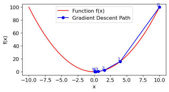
import numpy as np
import matplotlib.pyplot as plt

def f(x):  # Objective function
    return x ** 2

def f_grad(x):  # Gradient (derivative) of the objective function
    return 2 * x

def gd(eta, f_grad):
    x = 10.0  # initial solution
    results = [x]
    for i in range(5):
        x = x - eta * f_grad(x)
        results.append(float(x))
    return results
def show_trace(results, f):
    # Define the range of the plot based on the solutions
    n = max(abs(min(results)), abs(max(results)))
    f_line = np.arange(-n, n, 0.1)

    # Plot the function
    plt.plot(f_line, [f(x) for x in f_line], 'r-', label='Function f(x)')

    # Plot the solution path
    plt.plot(results, [f(x) for x in results], 'bo-', label='Gradient Descent Path')

    # Annotate each solution point with the iteration number
    for i, x in enumerate(results):
        plt.text(x, f(x), f'{i}', color='blue', fontsize=10,
                 ha='right', va='bottom')

    # Add labels and legend for better clarity
    plt.xlabel('x')
    plt.ylabel('f(x)')
    plt.legend()

    # Show the plot
    plt.show()
show_trace(gd(0.3, f_grad), f)
Batch GD for linear regression#
Recall the gradient vector of the loss function
GD step with fixed learning rate
This formula involves calculations over the full training set \(\mathbf{X}\) –> batch or full GD
An epoch means one complete pass of the training data set
# GDP data
import numpy as np
import pandas as pd
import matplotlib.pyplot as plt

df = pd.read_csv("https://github.com/ageron/data/raw/main/lifesat/lifesat.csv")

X = df['GDP per capita (USD)'].to_numpy()
y = df['Life satisfaction'].to_numpy()

def add_column(X):
    '''
    add the column of all 1's
    '''
    return np.concatenate(( np.ones((X.shape[0],1)), X.reshape(-1,1)), axis=1)
from sklearn.preprocessing import MinMaxScaler

minmax = MinMaxScaler()

X_minmax = minmax.fit_transform(X.reshape(-1,1))

Xcon = add_column(X_minmax)

print(Xcon[:5])
[[1.         0.        ]
 [1.         0.02459182]
 [1.         0.05709406]
 [1.         0.10290627]
 [1.         0.13473858]]
# Implementation of Batch GD

eta = 0.01  # learning rate
n_epochs = 1000
N = len(Xcon)  # number of instances

np.random.seed(3)
theta = np.random.randn(2, 1)  # randomly initialized model parameters

for epoch in range(n_epochs):
    gradients = 2 / N * Xcon.T @ (Xcon @ theta - y.reshape(-1,1))
    theta = theta - eta * gradients

print(theta)
[[5.54877943]
 [2.27673633]]
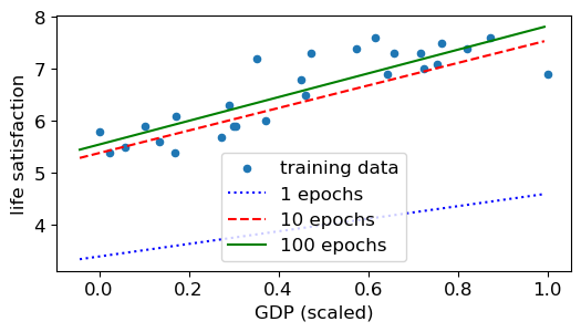
# Impact of eta (step size)
np.random.seed(3)
theta = np.random.randn(2, 1)  # randomly initialized model parameters

X_test = np.array([25000, 60000]).reshape(-1,1)
X_test_minmax = add_column(minmax.transform(X_test))

plt.scatter(X_minmax, y, s=20, label='training data')

eta= .1 # 0.001, 0.01, 0.1
for epoch in range(n_epochs):
    gradients = 2 / N * Xcon.T @ (Xcon @ theta - y.reshape(-1,1))
    theta = theta - eta * gradients
    if epoch == 1:
        plt.plot(X_test_minmax[:,1], X_test_minmax@theta , 'b:', label='1 epochs')
    elif epoch == 10:
        plt.plot(X_test_minmax[:,1], X_test_minmax@theta , 'r--', label='10 epochs')
    elif epoch == 100:
        plt.plot(X_test_minmax[:,1], X_test_minmax@theta , 'g-', label='100 epochs')
plt.legend()
plt.xlabel('GDP (scaled)')
plt.ylabel('life satisfaction')
plt.show()
Stochastic gradient descent (SGD) for linear regression#
The main problem with GD is that it uses the whole training set at every step
Consider a minibatch of size \(B=1\) and a selected sample \(\mathbf{x}_n^T\) from \(\mathbf{X}\) (row vector)
Given that \(N\) is the sample size and \(B\) is the batch size, in one epoch we update our model \(N/B\) times
n_epochs = 5
t0, t1 = 5, 50  # learning schedule hyperparameters

def learning_schedule(t):
    return t0 / (t + t1)

np.random.seed(42)
theta = np.random.randn(2, 1)  # random initialization

# Loop over the number of epochs (complete passes over the data)
for epoch in range(n_epochs):
    # Loop over individual data points
    for iteration in range(N): #(N/B, B=1)
        # Select a random index for the current data point
        random_index = np.random.randint(N)

        # Extract xi and yi
        xi = np.transpose(Xcon[random_index : random_index + 1])
        yi = y[random_index : random_index + 1]

        # Compute the gradient of the loss function
        gradients = 2 * xi @ (xi.T @ theta - yi)  # for SGD, do not divide by N

        # The learning schedule decreases the learning rate over time
        eta = learning_schedule(epoch * N + iteration)

        # Update the parameter vector (theta)
        theta = theta - eta * gradients

print(theta)
[[5.56898107]
 [2.27782555]]
Sklearn implementation of SGD for linear regression
https://scikit-learn.org/stable/modules/generated/sklearn.linear_model.SGDRegressor.html
Parameters
max_iter: epochs
learning_rate: constant or variable
n_iter_no_change: number of iterations with no improvement to wait before stopping fitting
# GDP data
from sklearn.pipeline import Pipeline
from sklearn.linear_model import SGDRegressor

X = df['GDP per capita (USD)'].to_numpy().reshape(-1,1)
y = df['Life satisfaction'].to_numpy()

pipe = Pipeline([('preprocess', MinMaxScaler()),
                 ('reg', SGDRegressor(random_state=42))])

pipe.fit(X, y)

print(pipe['reg'].intercept_, pipe['reg'].coef_)
[5.35324059] [2.47088247]
5. Nonlinear extension and regularization#
The linear model may not be a good fit for many problems
We can improve the fit by using a polynomial regression model of degree \(d\)
where \(\phi(x)=[1,x,x^2,\ldots,x^d]\)
This is a simple example of feature preprocessing/engineering
Benefit: linear function of parameters but nonlinear wrt input features
We can use sklearn.preprocessing.PolynomialFeatures to generate polynomial features
Use pipeline in sklearn to assemble several steps (preprocessing + estimator)
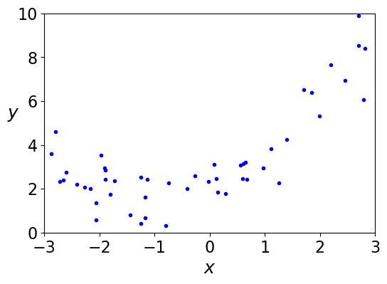
In the following, we generate a synthetic model of the form:
where the noise represents random variations added to simulate real-world data.
# Generate simulated data
import numpy as np
import matplotlib.pyplot as plt

np.random.seed(42)
plt.rcParams.update({'font.size': 16, "figure.figsize": (6,4)})

N = 50
X = 6 * np.random.rand(N, 1) - 3
y = 0.5 * X**2 + X + 2 + np.random.randn(N, 1)

plt.plot(X, y, "b.")
plt.xlabel("$x$", fontsize=18)
plt.ylabel("$y$", rotation=0, fontsize=18)
plt.axis([-3, 3, 0, 10])
plt.show()
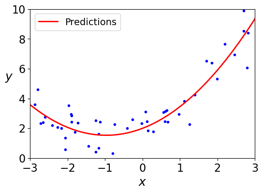
# train polynomial model
from sklearn.preprocessing import PolynomialFeatures
from sklearn.pipeline import Pipeline
from sklearn.linear_model import LinearRegression

pipe = Pipeline([
    ('poly', PolynomialFeatures(degree=2, include_bias=False)),
    ('regr', LinearRegression())])

pipe.fit(X, y) # training

X_new = np.linspace(-3, 3, 100).reshape(100, 1)
y_new = pipe.predict(X_new) # prediction

plt.plot(X, y, "b.")
plt.plot(X_new, y_new, "r-", linewidth=2, label="Predictions")
plt.xlabel("$x$", fontsize=18)
plt.ylabel("$y$", rotation=0, fontsize=18)
plt.legend(loc="upper left", fontsize=14)
plt.axis([-3, 3, 0, 10])
plt.show()
# Compare varying complexity levels

from sklearn.preprocessing import StandardScaler

for style, degree in (("g-", 40), ("b--", 2), ("r-+", 1)):
    polybig_features = PolynomialFeatures(degree=degree, include_bias=False)
    std_scaler = StandardScaler()
    lin_reg = LinearRegression()
    polynomial_regression = Pipeline([("poly_features", polybig_features),
                                      ("std_scaler", std_scaler),
                                      ("lin_reg", lin_reg)])
    polynomial_regression.fit(X, y)
    y_newbig = polynomial_regression.predict(X_new)
    plt.plot(X_new, y_newbig, style, label=str(degree))

plt.plot(X, y, "b.", linewidth=3)
plt.legend()
plt.xlabel("$x$", fontsize=14)
plt.ylabel("$y$", rotation=0, fontsize=14)
plt.axis([-3, 3, -10, 10])
plt.show()
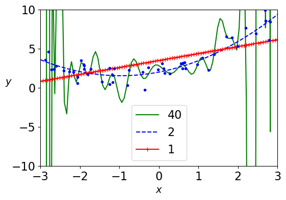
The bias-variance tradeoff#
A model’s generalization (or test) error can be decomposed into three components:
Bias: Error introduced by approximating a real-world problem, which may be complex, by a simplified model.
High bias models make strong assumptions about the data, potentially leading to underfitting, where the model fails to capture underlying patterns.
Variance: Error introduced by the model’s sensitivity to small fluctuations in the training set.
High variance models are overly sensitive to training data variations, leading to overfitting, where the model captures noise rather than the intended outputs.
Irreducible Error: Error inherent in the data itself, due to noise or other unpredictable factors, which cannot be reduced by any model.
Model flexibility and error relationship
As a model’s flexibility (complexity) increases, its training error typically decreases because it can fit the training data more closely.
However, the test error often follows a U-shaped curve:
With low flexibility, both training and test errors are high due to underfitting.
With moderate flexibility, test error decreases as the model captures the underlying data patterns.
Beyond a certain point, increasing flexibility leads to overfitting, causing test error to rise even as training error continues to decline.
This balance between bias and variance is known as the bias-variance tradeoff. Achieving optimal model performance involves finding the right level of complexity that minimizes test error by appropriately balancing bias and variance.

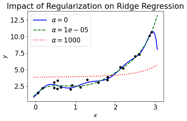
Regularization#
Regularization adds a penalty term to the model’s loss function to discourage excessive complexity.
Common regularization techniques:
L1 Regularization (Lasso): Adds the sum of the absolute values of coefficients as a penalty.
L2 Regularization (Ridge): Adds the sum of the squares of coefficients as a penalty.
Elastic Net: Combines L1 and L2 penalties.
By discouraging large weights, it prevents the model from overfitting small variations or noise in the training data.
Mathematical representation
* $\lambda\geq 0$ is the regularization parameter (i.e., hyperparameter) and $C(\boldsymbol{\theta})$ is some form of model complexity.
* We can quantify complexity using the L2 regularization formula, i.e., the sum of the squares of all weights
# Synthetic/Simulated Data (Ridge Regression or L2)
from sklearn.linear_model import Ridge
import numpy as np
import matplotlib.pyplot as plt
from sklearn.pipeline import Pipeline
from sklearn.preprocessing import PolynomialFeatures, StandardScaler

# Seed for reproducibility
np.random.seed(42)

# Generate synthetic data with a cubic relationship
N = 20
X = 3 * np.random.rand(N, 1)
y = 2 + 0.5 * X**3 - 0.8 * X**2 + X + np.random.randn(N, 1) / 2  # Cubic function with noise
X_new = np.linspace(0-0.05, 3+0.05, 100).reshape(100, 1)

# Regularization strengths to explore
alphas = (0, 10**-5, 1000)

# Iterate through different alpha values and plot the results
for alpha, style in zip(alphas, ("b-", "g--", "r:")):  # zip aggregates alphas and styles
    model = Pipeline([
        ("poly_features", PolynomialFeatures(degree=10, include_bias=False)),  # 10th degree polynomial
        ("std_scaler", StandardScaler()),  # Standardize features
        ("regul_reg", Ridge(alpha=alpha)),  # Ridge regression with specified alpha
    ])
    model.fit(X, y)
    plt.plot(X_new, model.predict(X_new), style, linewidth=2, label=r"$\alpha = {}$".format(alpha))

# Plot the original data
plt.plot(X, y, "k.", markersize=10)  # Original data points
plt.legend()
plt.xlabel("$x$", fontsize=14)
plt.ylabel("$y$", fontsize=14)
plt.title("Impact of Regularization on Ridge Regression")
plt.show()
Synthetic data generation for comparing L1 (Lasso) vs L2 (Ridge):
The
make_regressionfunction is used to create a data set for regression tasks:n_samples=50: 50 data points are generated.n_features=5: The data has 5 features.n_informative=2: Out of the 5 features, only 2 are truly informative (affect the target variable).noise=1: Adds Gaussian noise to the target variable to make the problem more realistic.effective_rank=2: Introduces correlations between features by generating a low-rank design matrix.coef=True: Returns the coefficients of the underlying true model.
import numpy as np
from sklearn.linear_model import Lasso, Ridge
from sklearn.datasets import make_regression
import matplotlib.pyplot as plt

# Generate synthetic data with redundant features
np.random.seed(5)
X, y, coefficients = make_regression(
    n_samples=50,  # Number of samples
    n_features=5,  # Total features
    n_informative=2,  # Only 2 features are informative
    noise=1,  # Add some noise
    effective_rank =2,
    coef=True,  # Return the coefficients for the true model
)

print(coefficients)
[85.84989327 0. 25.73873511 0. 0. ]
# Apply Lasso Regression
lasso = Lasso(alpha=0.1)  # L1 regularization strength
lasso.fit(X, y)

# Apply Ridge Regression
ridge = Ridge(alpha=0.1)  # L2 regularization strength
ridge.fit(X, y)

# Plotting side-by-side comparison
width = 0.25  # Width of the bars
x_indices = np.arange(len(coefficients))  # Indices for features

plt.figure(figsize=(8, 4))

# Plot True coefficients
plt.bar(x_indices - width, coefficients, width=width, label="True Coefficients", color='gray')

# Plot Lasso coefficients
plt.bar(x_indices, lasso.coef_, width=width, label="Lasso Coefficients (L1)", color='blue')

# Plot Ridge coefficients
plt.bar(x_indices + width, ridge.coef_, width=width, label="Ridge Coefficients (L2)", color='orange')

# Add labels and formatting
plt.axhline(0, color='black', linestyle='--', linewidth=0.8)
plt.xlabel("Feature Index")
plt.ylabel("Coefficient Value")
plt.title("Lasso vs Ridge: Side-by-Side Comparison of Coefficients")
plt.xticks(x_indices)
plt.legend()
plt.show()
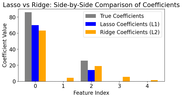
When features are highly correlated (as happens with
effective_rank=2), Ridge struggles to distinguish between them, which can result in suboptimal generalization and interpretation.Lasso regression performs feature selection by setting some coefficients to zero. It eliminates redundant or less important features entirely.
Recommended Reading#
Chapters 3 and 5 of An Introduction to Statistical Learning With Applications in Python: https://www.statlearning.com/
Chapter 4 of Hands-on Machine Learning with Scikit-Learn, Keras and TensorFlow: ageron/handson-ml3
Chapter 11 of Probabilistic Machine Learning: An Introduction: https://probml.github.io/pml-book/book1.html